PCCF Guide

In this tutorial, we will use the Postal Code Conversion File (PCCF) to match postal codes to dissemination areas in order to incorporate additional neighbourhood-level demographic data into your dataset.

There are multiple postal code products that can accomplish this task. For an overview, see our general PCCF page https://mdl.library.utoronto.ca/collections/numeric-data/census-canada/postal-code-conversion-file. In this tutorial we will use the standard PCCF file which uses a Single Link Indicator (SLI) to assign a postal code to the geographic area with the majority of dwellings. There are scenarios where it would be better to use the PCCF+ file, which uses a population-weighted random allocation to assign a postal code to a geographic area. It tends to work better when your postal codes are rural or when the “vintage” of your postal codes pans more than one census. See this guide Statistics Canada created for more information on selecting a PCCF product that meets your needs.

This guide contains two parts and an appendix. In part A, you will start with the postal codes from your dataset and use the PCCF to assign Statistics Canada standard geographic identifiers to your postal codes. In part B, you will enrich your final dataset from part A with census data. This guide shows you how to complete these steps using SPSS, and the appendix contains additional code to run parts A and B using R, SAS, Stata or Python.

TABLE OF CONTENTS
Part A: Use the PCCF to assign standard geographic codes/names to your postal codes
Part B: Enrich your dataset with census data

APPENDIX
SAS Code
R Code
Stata Code
Python Code
SPSS Code

Part A: Use the PCCF to assign standard geographic codes/names to your postal codes

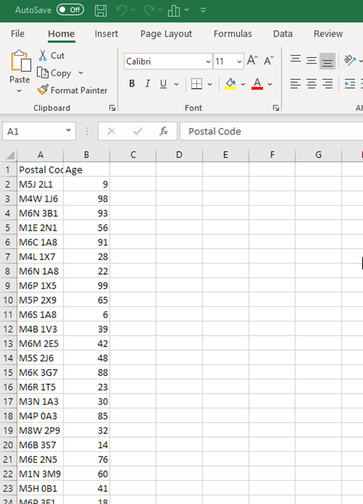
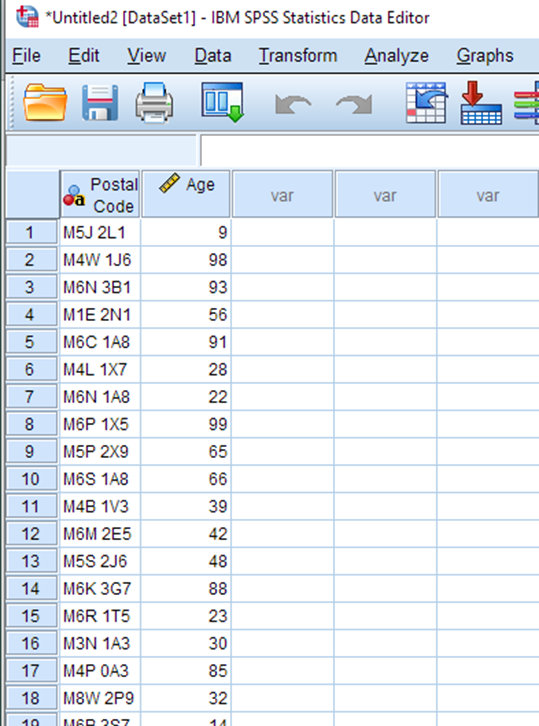
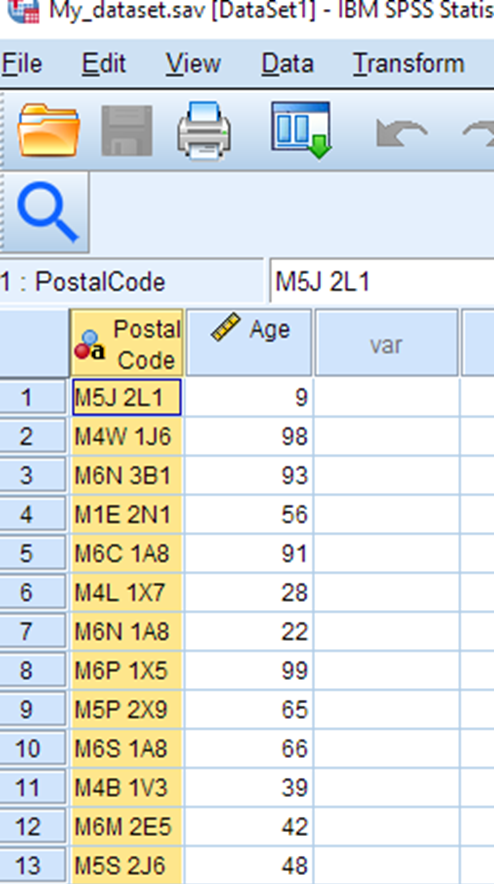
Start with a dataset that includes postal code level data. Make sure you have a separate field for the postal code. You must have full 6-digit postal codes to work with the standard PCCF file (if you have 3, 4 or 5 digits of the postal code, you can use the PCCF+). For this tutorial, we will demonstrate using this sample dataset. It contains two columns, postal code (consisting of 50 randomly generated postal codes within Toronto) and age (consisting of 50 randomly generated values between 1 and 99). As you work, imagine that this dataset represents the participants in a study you conducted. Or, use your own data.
Download the sample dataset: https://maps.library.utoronto.ca/workshops/PCCF/My_dataset.csv
Bring your postal code data into SPSS. In this exercise, we will be loading in a csv file, but SPSS can accommodate many file types. If you run into difficulties loading your own data into SPSS, contact us for assistance.
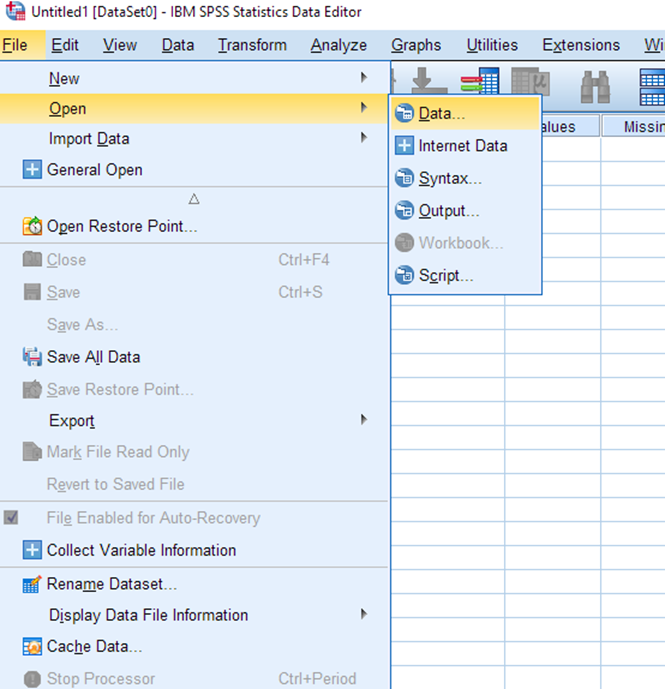
Open SPSS on your computer. From the File menu, choose Open > Data.
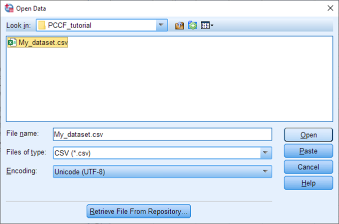
Select Files of type: CSV and then browse to your dataset (or wherever you saved the sample file provided for this tutorial). Select Open.
The Text Import Wizard pops up. Our sample data is a very simple CSV file with only one column, so we can mostly just skip through this wizard without changing anything. (If you are loading your own dataset, make the appropriate choices for your dataset at each step).
For steps 1-3, no changes are required. Select Next.
For step 4, ensure Comma is selected and Space is not selected. Select Next.
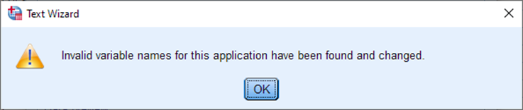
For step 5, You will get a pop-up that says it found invalid variable names. This is because spaces are not allowed in variable names (column headers) in SPSS. Select OK and the wizard will remove the space in our variable name for us (to ‘PostalCode’). Select Next.
On step 6, no changes are required. Select Finish.
You now have your data loaded into SPSS.
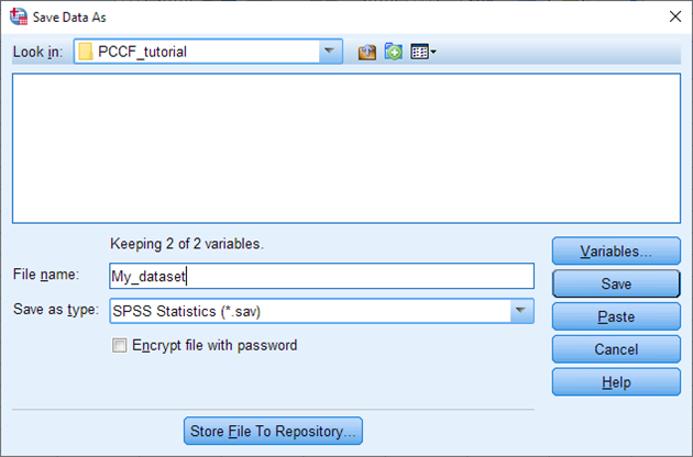
Save the dataset by selecting File > Save As. Save it as a .sav file.
Leave the file open in SPSS for now, we will return to it shortly.
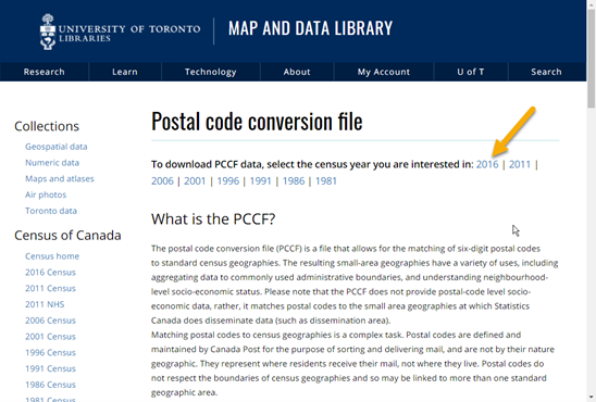
Download the PCCF dataset from the MDL website: https://mdl.library.utoronto.ca/collections/numeric-data/census-canada/postal-code-conversion-file.
Choose the census year of interest.
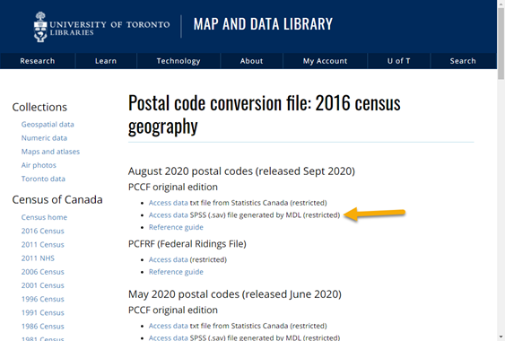
Choose the SPSS version of the file (the Map & Data Library has already done the work of preparing the original file for use in SPSS!)
Please carefully read through the end-user license agreement.
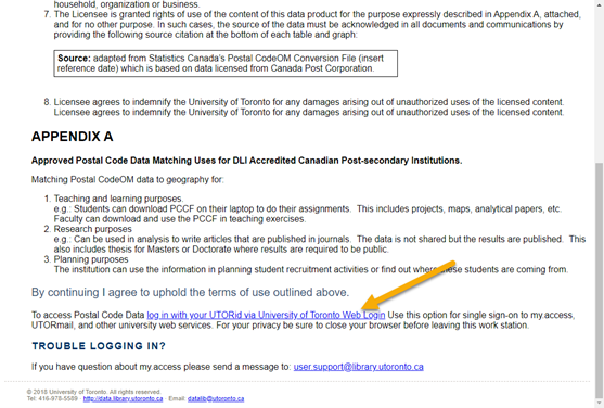
At the bottom of the page, click the link to authenticate with your UTORid. The download will then start automatically.
If you wish, move the file from your Downloads folder to some location where you will find it again later.
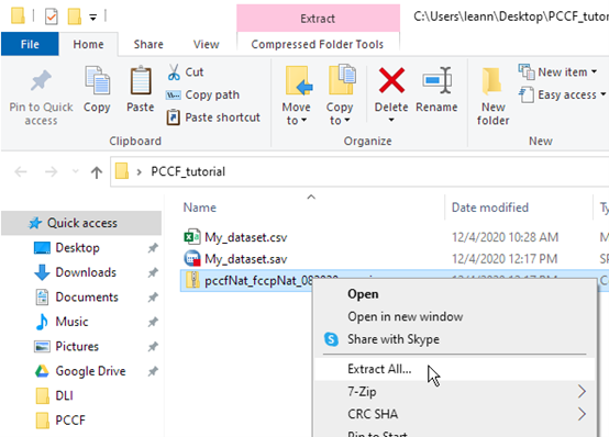
The download is a compressed file which must be uncompressed (or “unzipped”). Right-click on the file and choose Extract All. On a Mac you can simply double-click on the file.
Open the PCCF data in SPSS. You can do this from within SPSS, by selecting File > Open > Data again. Another option when you are opening a file that is already in the native SPSS format (.sav) is to simply browse to the file on your computer and double-click it. This will cause it to open in SPSS automatically.
Note: You may see the following message:
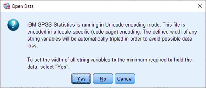
You can answer “Yes”.
You should now have two SPSS datasets open on your computer:
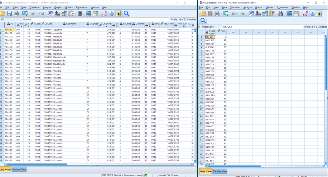
Prepare your own postal code dataset for a merge. To merge two datasets, you need to have a common column to match on. In this case, we want to match on the postal code field. Ultimately, we want to keep one row for every record in our dataset (e.g. the 50 postal codes in My_dataset) and add in the data from the PCCF file columns (the province, census division, census subdivision, census tract, dissemination area etc. codes that match our postal codes).
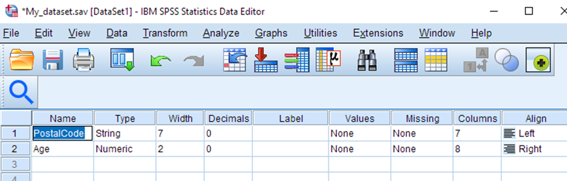
Have a look at the two postal code fields in our two datasets. You can see that they are formatted differently. In the PCCF, it is a 6-character alphanumeric field, whereas in our sample data it is a 7-character alphanumeric field with a space in it. We will need to remove the space from our data before we can proceed.
Select the PostalCode column in the sample dataset.
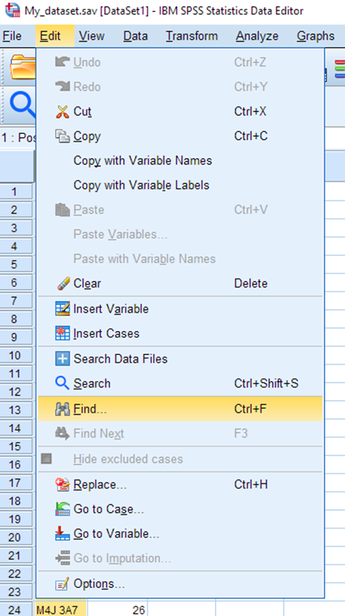
In the Edit menu, select Find…
Choose the Replace tab. In the Find box, type a space. Leave the Replace with box as it is. Select Replace All.
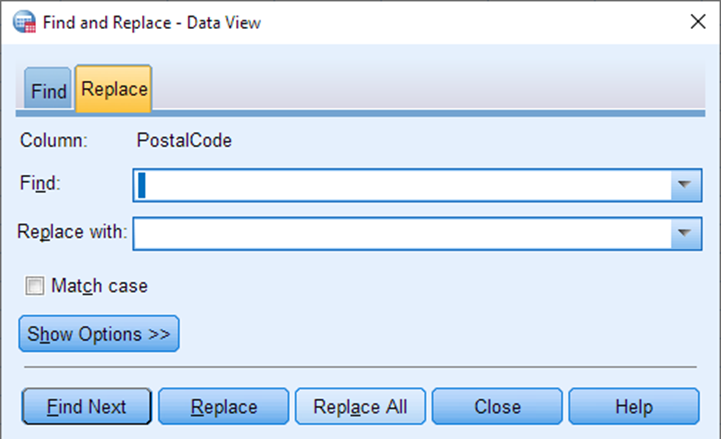
50 replacements will be made. Close the dialog when finished.
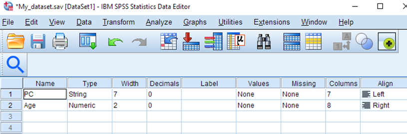
The other issue we need to address is that SPSS expects the fields being merged to have the same variable name. In our sample data, let’s change the PostalCode variable to be named PC instead, to match the PCCF file.
While looking at your sample dataset, select Variable View. In the Name column, overwrite the name of the PostalCode column to PC.
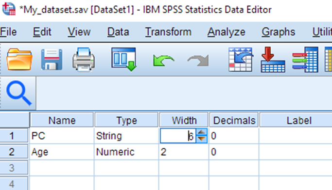
While we are at it, let’s also change the width of the PC variable to 6, since the data only takes up 6 characters now that the spaces have been removed.
If you are working with your own data, perform any further data cleanup necessary to ensure your postal codes are formatted the same as those in the PCCF file. Save your dataset.
Prepare the PCCF dataset for a merge. Because of the nature of postal codes, it is common for postal codes to match more than one standard census geography (e.g. a postal code overlaps 2 dissemination areas). The PCCF provides a field called the Single Link Indicator (SLI) which can be used to select one matching geography (the one where the most dwellings are located). Note: if you need a more nuanced approach to selecting which geography to match your postal codes to, consider using the PCCF+ instead.
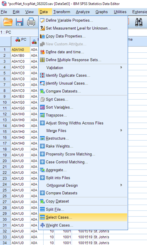
We will select only those records where the SLI value = 1 so that we will not end up with duplicate records.
From the Data menu, choose Select Cases.
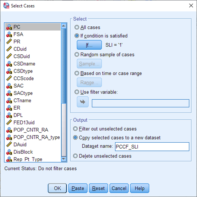
The Select Cases dialog appears. Choose If condition is satisfied, and select the If… button.
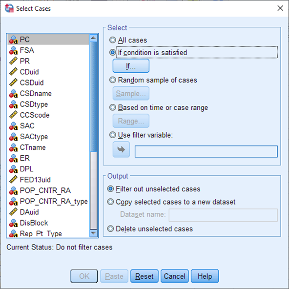
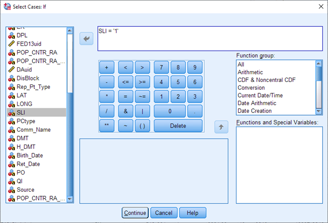
Select Single link indicator from the variable list, then click the arrow to bring it over into the expression box. Then type = ‘1’. (The number must be surrounded by quotation marks because the variable is coded as a String variable). Select Continue.
Under Output, choose Copy selected cases to a new dataset. Call it PCCF_SLI. Select OK.
If you examine the new dataset PCCF_SLI, you’ll notice there are now roughly half as many records (rows). Save this new dataset, we will work with it from now on. You can close the original PCCF file.
Now we are ready to merge the two files. We will show the steps to do this using the Merge dialog in the SPSS GUI. However, this dialog is confusingly organized and does not provide all the merge options that are actually available in SPSS. For that reason, you may wish to consider performing merges in SPSS using SPSS syntax (code). The steps to do this are located in the final appendix of this guide (called ‘SPSS code for merges’).
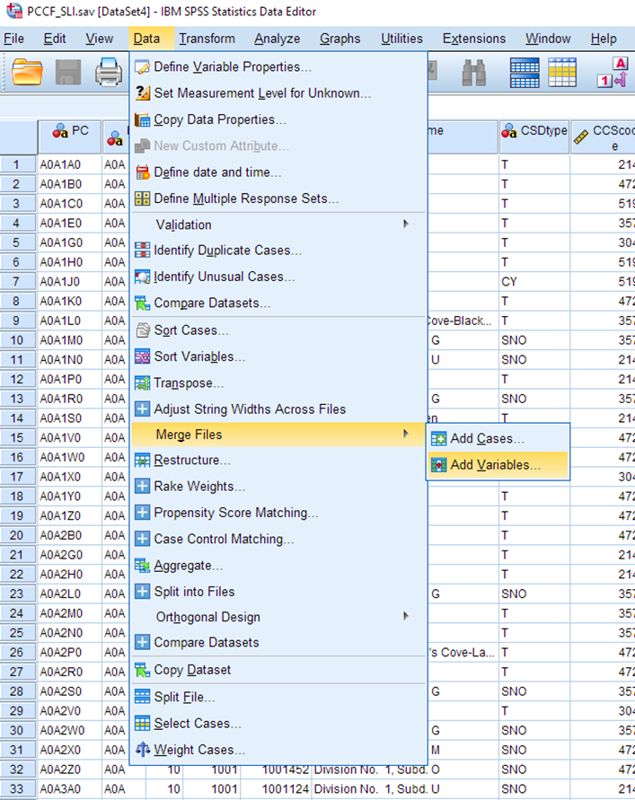
To do this using the Merge dialog: from within the PCCF_SLI dataset, choose Data > Merge Files > Add Variables…
Next select your own dataset, which should be listed as an open dataset. Select Continue.
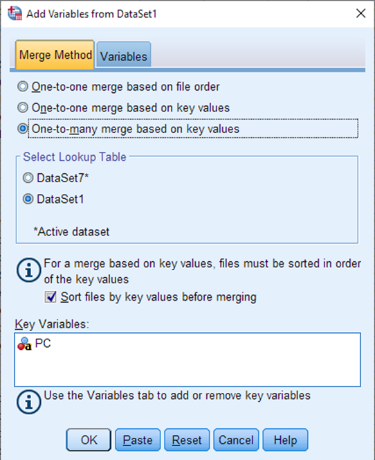
In the next window, on the Merge Method tab, select “One-to-many merge based on key values”. For Select Lookup Table, select whichever one represents the sample dataset (the dataset numbers will vary depending on whether you have closed and opened your data files multiple times during your session). Select Sort files by key values before merging. Because each dataset has a column named PC, SPSS will have already populated the variable PC as the key variable.
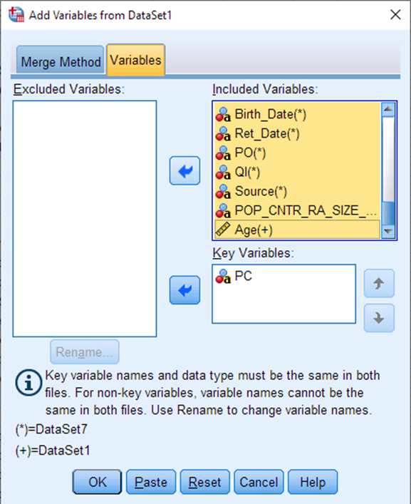
Click on the Variables tab at the top. Let’s remove some extraneous PCCF columns at this point. Let’s say you are only interested in census tracts and dissemination areas (we already know all our data is within Toronto, so any larger geographies aren’t very helpful to us). Use Shift+select to highlight all of the variables in the Included box, then click the arrow to move them over to the Excluded box.
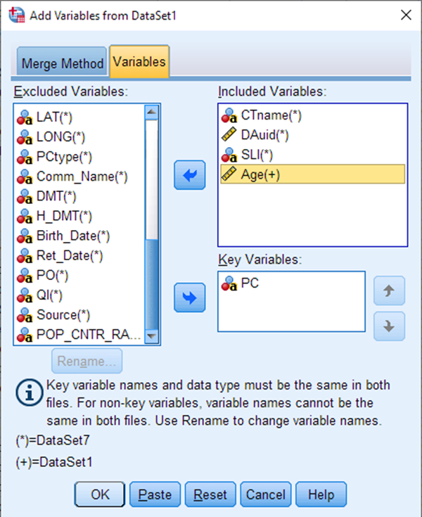
Now choose the variables CTname, DAuid, SLI and Age, and move them back over to the Included Variables box. Select OK.
Your merge is now complete. You’ll notice that initially there appear to be no values in the Age column. This is because we only had Age values for 50 out of the 1.8 million postal codes that are in this file. We need to remove the extraneous postal codes from the file now, so we are left with only our own postal codes of interest.
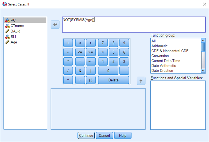
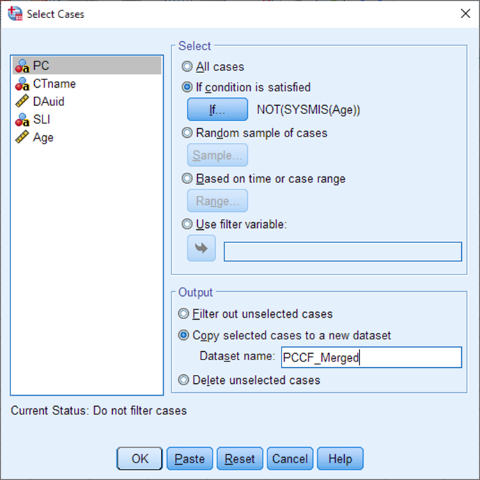
In the Data menu, choose Select Cases. Choose If condition is satisfied, then select the If… button. In the expression builder box, type the following statement: NOT(SYSMIS(Age)). This should select all rows where the age value is not missing (i.e. all those which have an age value). NOTE: This will only work if you have a column in your dataset where there are values in every cell (no missing values). If that is not the case, you will need to perform your merge using SPSS syntax instead – see the code sample included in the appendix at the end of this guide (called ‘SPSS code for merges’). If you have a column of data without missing values, you can continue with these steps.
Select Continue.
Choose Copy selected cases to a new dataset, and give it the name PCCF_Merged. (You could also choose to Delete the unselected cases from your existing dataset, but only do this if you are very confident your expression will do what you expect it to!). Select OK.
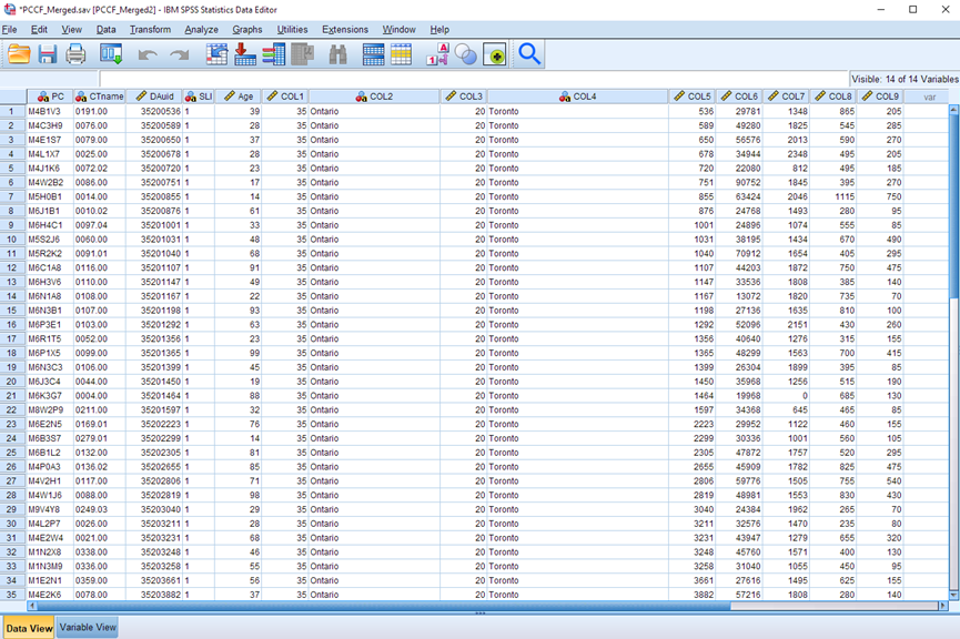
Ta da! You now have your original data columns plus the codes for the census tract and the dissemination area that matches your postal codes of interest. In the next part of this tutorial, we will use the DAuid to pull in some census data to enrich this dataset.
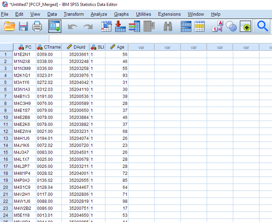
Save this data file as PCCF_Merged.sav.

Part B. Enrich your dataset with census data

In this section of the guide, we will incorporate census data to the dataset created in Part A, by merging on Statistics Canada geographic identifiers.

We need to download some census data at the Dissemination Area level of geography. Each Dissemination area will have a unique ID that will be a match to the DAuid column we merged in from the PCCF in Part A.
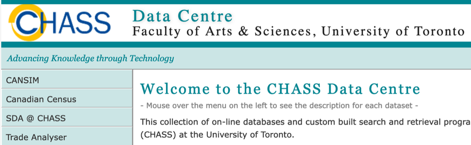
We can download the census dataset from the CHASS Data Centre website To access the data from CHASS, you need to login using your UTORid using the following link: https://login.library.utoronto.ca/index.php?url=http://dc.chass.utoronto.ca/
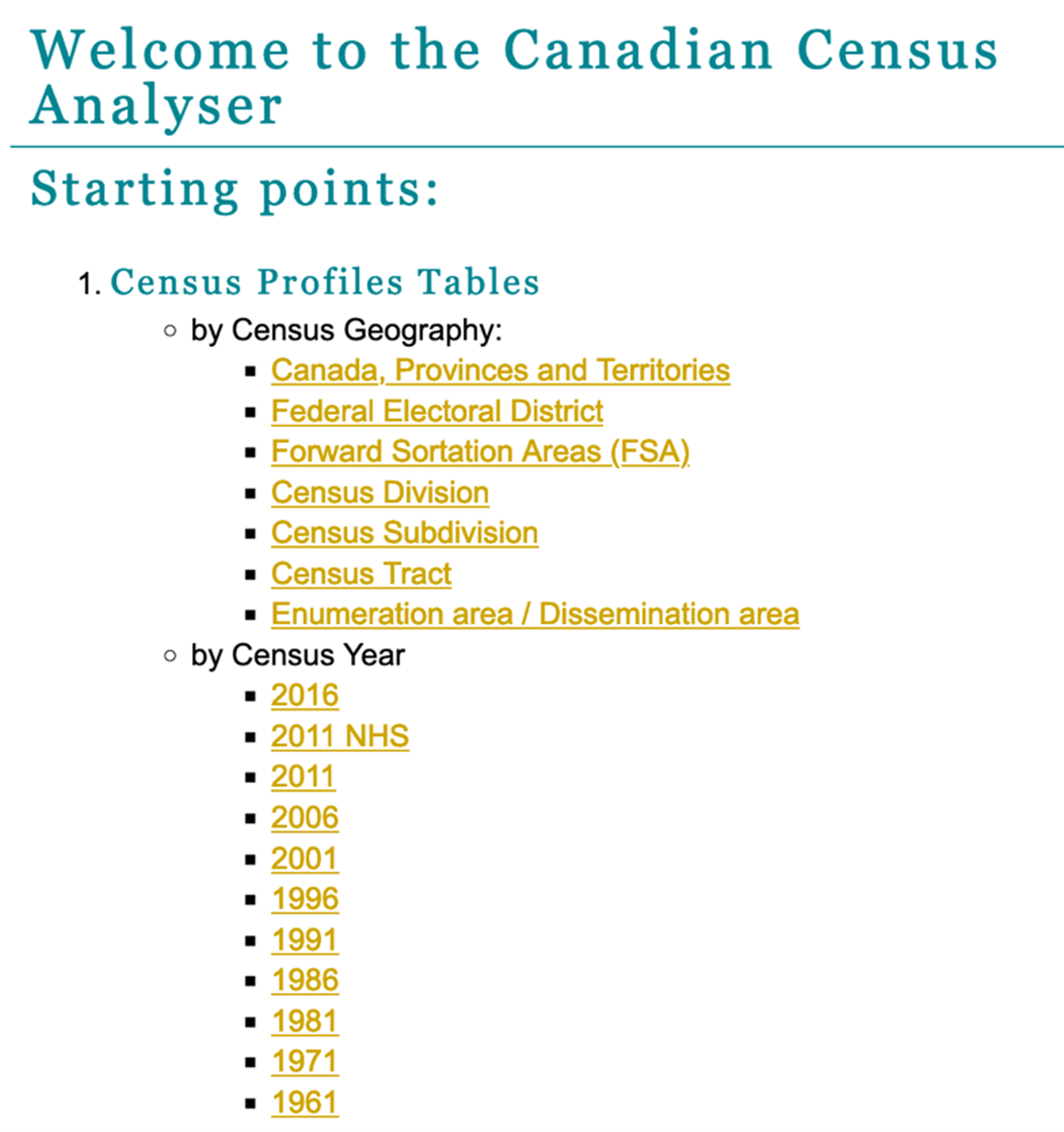
After you login, you will be directed to the CHASS Data Centre homepage. From the menu on the left-hand side, select Canadian Census.
This will take you to the Census Analyser page. We will need to select the census profiles by census year and census geography. We will select our census profiles by census year first for this guide. Select 2016 under by Census Year.
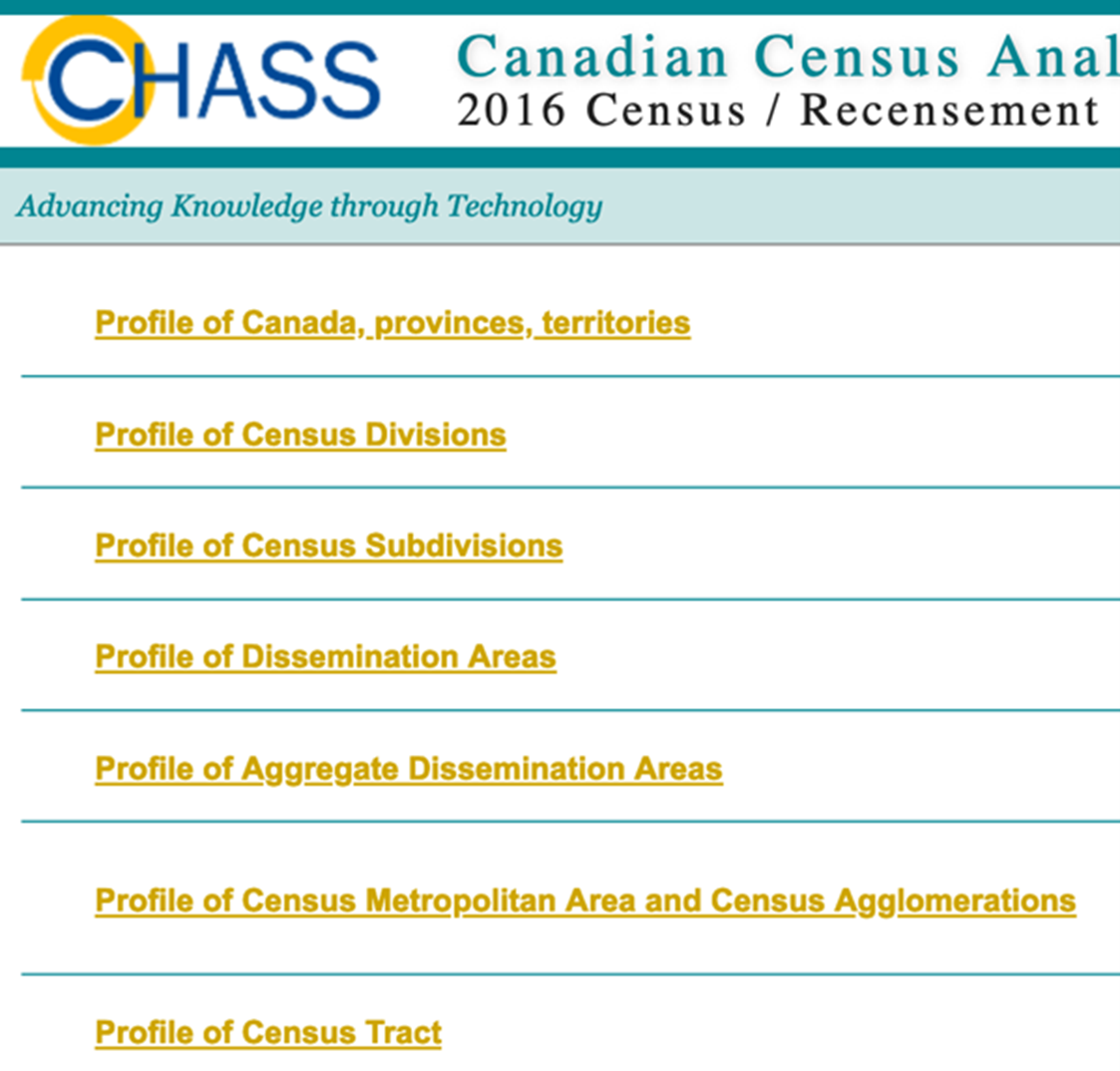
Then we select the census geography. Select Profile of Dissemination Areas.
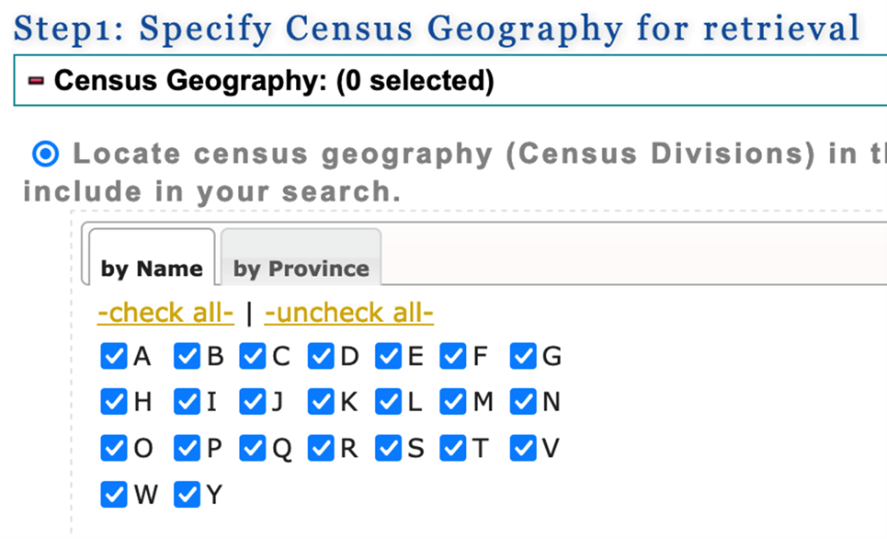
This will direct you to a page where you can make additional choices to make your census profile table. In step 1, you can select a subset of regions or select all. For this guide, we will select “check all”.
In step 2, you can select the census variables that you are interested in. (Note: you may need to scroll way down the page before you see step 2).The variables are grouped by topic under the topic tabs (eg. Population and dwellings, Age & sex etc). You will find the list of variables under the tabs. To select a variable, click on the check box to the left of the variable description.
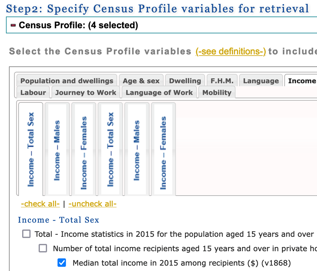
For this guide, we select the following four variables (you can choose others based on your own research interest):
1. Income - Total Sex / Total - Income statistics in 2015 for the population aged 15 years and over in private households - 100% data / Number of total income recipients aged 15 years and over in private households - 100% data / Median total income in 2015 among recipients ($) (v1868)
2. Housing - Total Sex / Total - Owner households in non-farm, non-reserve private dwellings - 25% sample data / Median monthly shelter costs for owned dwellings ($) (v3942)
3. Education - Total Sex / Total - Highest certificate, diploma or degree for the population aged 15 years and over in private households - 25% sample data (v4920)
4. Education - Total Sex / Total - Highest certificate, diploma or degree for the population aged 15 years and over in private households - 25% sample data / Postsecondary certificate, diploma or degree / University certificate, diploma or degree at bachelor level or above (v4929)
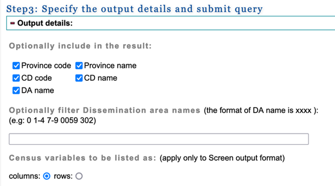
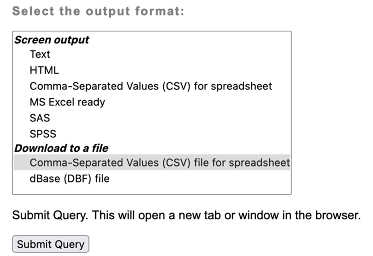
Scroll down to step 3. Here, you can select the geographic variables to be included in the census dataset and the output data format to download the census dataset.
Check all 5 of the geographic variables. In the Select the output format box, under Download to a file, we select Comma-Separated Values (CSV) file for spreadsheet to download the census dataset as a CSV file. Select Submit Query.
And finally, we click on Submit Query.
The wizard might take a few minutes to complete the query. When the data request is complete, you will be provided with two links. One to download the data file and another one to download a file with descriptions of the column names in the first data file (known as the “header file”).
Right-click on the link next to Data file to download the census dataset. Choose Save Link As… We save this data file as census2016.csv.
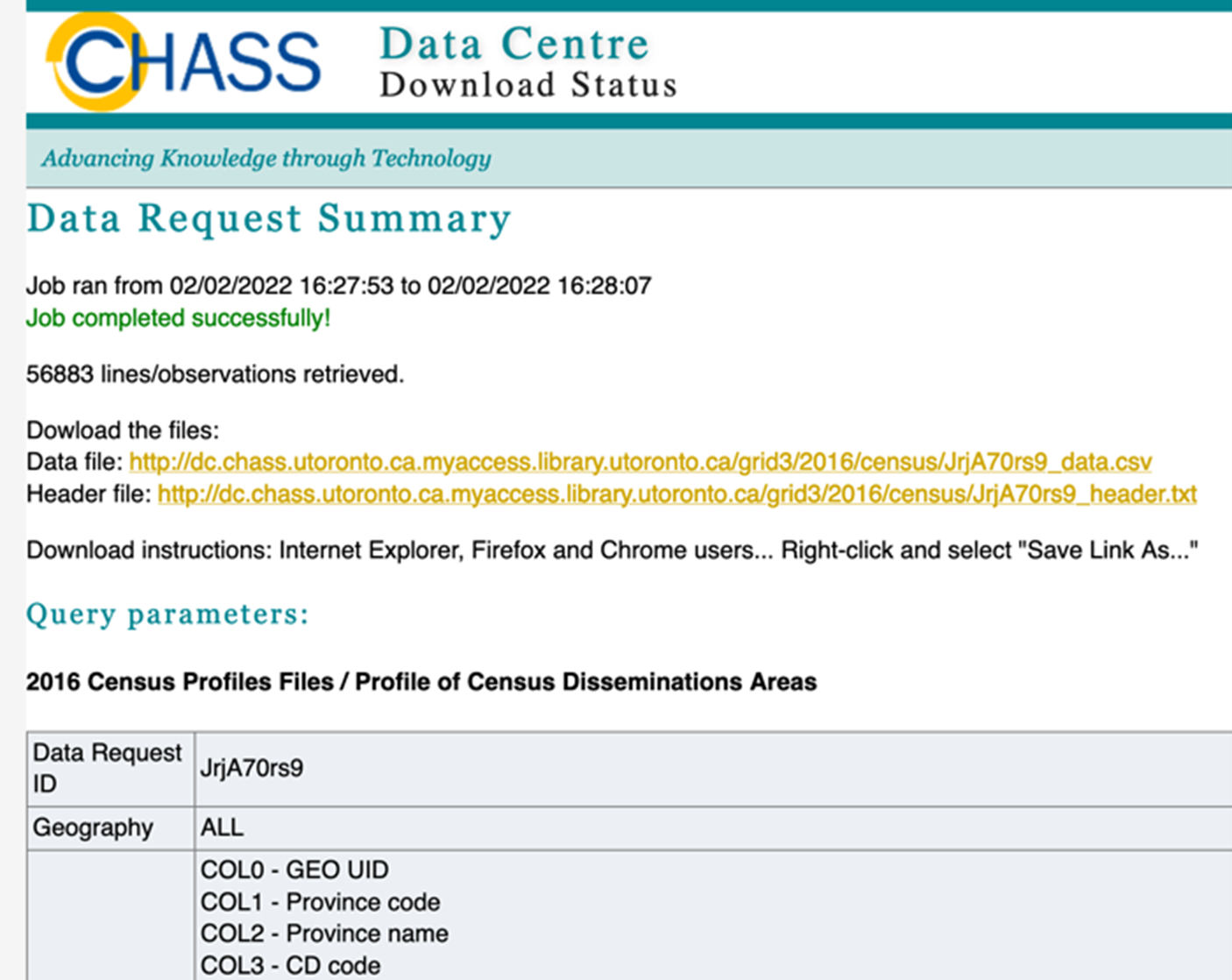
You will also need a copy of the header file with the descriptions of the column names (otherwise you won’t know what data is in what column later). Right-click on the header file link and choose Save Link As… We save this data file as ColumnHeaders.txt. We will make use of it in a future step.
Now we will enrich our postal code data with the census data we just downloaded. You should already have your postal code dataset open in SPSS (called PCCF_Merged). Let’s load the census data into SPSS next, so we can work with it.
From the File menu, choose Open > Data. Select Files of type: CSV and then browse to the location you saved the census dataset. Select the dataset and then select Open.
The Text Import Wizard pops up. Similar to when you used this Wizard earlier, you don’t need to alter much:
- For steps 1-3, no changes are required. Select Next.
- For step 4, ensure Comma is selected and Space is not selected. Select Next.
- For step 5, no changed are required. Select Next.
- For step 6, no changes are required. Select Finish.
You now have your data loaded into SPSS. It should look something like this:
Save a copy of this file as census2016.sav.
We next need to merge PCCF_Merged.sav with census2016.sav. As with our merge in part A, we need a common column to match on. This time, we will match on the unique ID number for dissemination areas (the geographic units we downloaded our census data at). In the PCCF_Merged.sav dataset, the column is called DAuid and is an 8-digit numeric variable. In census2016.sav, the comparable column is COL0 – according to your ColumnHeaders doc this column is actually called “GEO UID”, and if you look at its variable information, you will see that it is also an 8-digit numeric variable. (Side note: We also downloaded a column called “DA name” which may seem tempting, but that is a 4-digit number which represents the last 4 digits of the full unique ID. The “DA name” column is not unique across all of Canada and so cannot be used here).
Since the data types for our two columns are the same, the only edit we need to make before merging is to make the column names match. In the census2016 dataset, select Variable View. Change COL0 to DAuid. Then save the dataset.
Now we are ready to merge the files. Within the PCCF_Merged dataset, choose Data > Merge Files > Add Variables…
Next select the census2016 dataset, which should be listed as an open dataset. Select Continue.
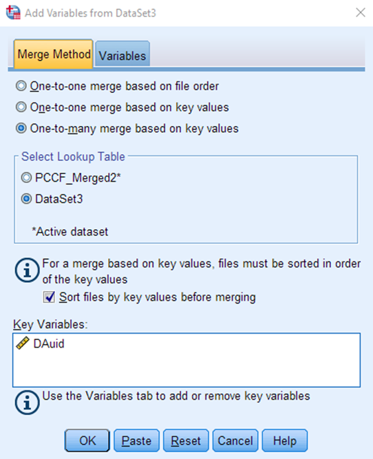
In the next window, on the Merge Method tab, select “One-to-many merge based on key values”. For Select Lookup Table, select whichever one represents the census dataset (the dataset numbers will vary depending on whether you have closed and opened your data files multiple times during your session). Select Sort files by key values before merging. Because each dataset has a column named DAuid, SPSS will have already populated the variable DAuid as the key variable. Select OK.
Your merge is now complete.
You will likely wish to switch to Variable View and update the variable names & labels to be more descriptive (use the ColumnHeader.txt file as a guide).
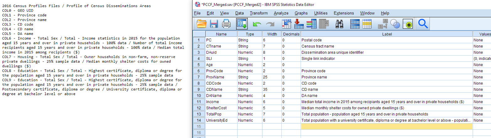
Don’t forget to save your file when you are finished!

Appendix

The SAS, R, Stata and Python code to accomplish the steps in part A and part B can be found below. The datasets used in the code are My_dataset.csv, the PCCF file and the census file. You need to follow the instructions in the guide to download the PCCF and the census datasets.

Key points to keep in mind about these statistical programs:

R is case sensitive
SAS is NOT case sensitive. Each line OF CODE ends with a semi-colon.
Stata is case sensitive

SAS CODE

* PCCF GUIDE;

* Instruction: 
*          - Replace the data file paths below with the respective file paths on your computer;

* Part A: Use the PCCF to assign standard geographic data to your postal codes;

* STEP 1: Import datasets;

* Import your dataset;
proc import out=work.mydataset
                           datafile="H:\PCCF Guide\Data\My_dataset.csv" 
                           dbms=csv replace;
         getnames=yes;
         datarow=2;
run;

* Import the PCCF file;
proc import out=work.pccf 
                           datafile="H:\PCCF Guide\Data\pccfNat_fccpNat_082021csv.csv"
                           dbms=csv replace;
         getnames=yes;
         datarow=2;
run;

* STEP 2: Prepare for merge;

* Keep only the postal codes that have a Single Link Indicator (SLI) value of 1 in pccf; 
data pccf; set pccf; if sli=1; run;

* Rename the postal code variables in mydataset and pccf pcode;
data mydataset; set mydataset; rename postal_code = pcode; run;
data pccf; set pccf; rename pc = pcode; run;

* Remove the single space in pcode in mydataset; 
data mydataset; set mydataset; pcode = compress(pcode); run;

* STEP 3: Merge datasets mydataset and pccf;

* Sort each dataset by the pcode variable;
proc sort data=mydataset; by pcode; run;
proc sort data=pccf; by pcode; run;

* Combine the two datasets by matching the pcode variable and only keep your postal codes;
data mydatasetpccf;
        merge mydataset (in=x) pccf;
        by pcode;
        if x=1;
run;

* STEP 4: Export mydatsetpccf;

* Create a libname to point to your output folder;
libname folder "H:\PCCF Guide\Data";

* Save mydatasetpccf as a SAS dataset in your output folder;
data folder.mydatasetpccf; set work.mydatasetpccf; run; 

* Export mydatasetpccf to CSV in your output folder;
proc export data=work.mydatasetpccf
                            outfile="H:\PCCF Guide\Data\mydatasetpccf.csv"
                            dbms=csv replace;
run;

* Part B: Adding census data; 

* Step 1: Import datasets;

* Import mydatasetpccf if you haven't run Part A;
proc import out=work.mydatasetpccf 
                           datafile="H:\PCCF Guide\Data\mydatasetpccf.csv" 
                           dbms=csv replace;
  getnames=yes;
  datarow=2;
run;

* Import the census data file;
proc import out=work.census
                           datafile="H:\PCCF Guide\Data\census2016.csv" 
                           dbms=csv replace;
  getnames=yes;
  datarow=2;
run;

* Step 2: Prepare for merge;

* Rename the col0 variable to dauid in census to match mydatasetpccf;
data census; set census; rename col0 = dauid; run; 

* Convert the data type of dauid from character to numeric in census to match mydatasetpccf;
data census; set census; dauid2 = input(dauid, 10.); drop dauid; rename dauid2=dauid; run;

* Step 3: Merge datasets mydatasetpccf and census;

* Sort each dataset by dauid;
proc sort data=mydatasetpccf; by dauid; run; 
proc sort data=census; by dauid; run; 

* Combine the two datasets by matching the dauid variable and only keep your DAs;
data mydataset2;
        merge mydatasetpccf(in=x) census;
        by dauid;
        if x=1;
run; 

* STEP 4: Export mydataset2; 

* Create a libname to point to your output folder;
libname folder "H:\PCCF Guide\Data";

* Save mydataset2 as a SAS dataset in your output folder;
data folder.mydataset2; set work.mydataset2; run;

* Export mydataset2 to CSV in your output folder;
proc export data=work.mydataset2
                           outfile="H:\PCCF Guide\Data\My_dataset2.csv"
                           dbms=csv replace;
run;

R Code

# PCCF GUIDE
# Instruction: 
# - Replace the data file paths below with the respective file paths on your computer.

# Part A: Use the PCCF to assign standard geographic data to your postal codes

# STEP 1: Import datasets
# Note: Change all backslashes to forward slashes
# Import your dataset
mydataset <- read.csv("H:/PCCF Guide/Data/My_dataset.csv")
# Import the PCCF file
pccf <- read.csv("H:/PCCF Guide/Data/pccfNat_fccpNat_082021csv.csv")

# STEP 2: Prepare for merge
# Keep only the postal codes that have a Single Link Indicator (SLI) value of 1 in pccf
pccf <- subset(pccf, SLI==1)
# Rename the postal code variables in mydataset and pccf pcode
names(mydataset)[names(mydataset)=="Postal.Code"] <- "pcode"
names(pccf)[1] <- "pcode"
# Remove the single space in pcode in mydataset
mydataset$pcode <- gsub(" ", "", mydataset$pcode) 

# STEP 3: Merge datasets mydataset and pccf
# Combine the two datasets by matching the pcode variable and only keep your postal codes
mydatasetpccf <- merge(mydataset, pccf, by="pcode", all.x=TRUE)

# STEP 4: Export mydatsetpccf 
# Export mydatasetpccf to CSV in your output folder
write.csv(mydatasetpccf,"H:/PCCF Guide/Data/mydatasetpccf.csv", row.names=FALSE)

# PART B: Adding census data

# Step 1: Import datasets
# Note: Change all backslashes to forward slashes
# Import mydatasetpccf if you haven't run Part A
mydatasetpccf <- read.csv("H:/PCCF Guide/Data/mydatasetpccf.csv")
# Import the census data file
census <- read.csv("H:/PCCF Guide/Data/census2016.csv")

# Step 2: Prepare for merge
# Rename the DAuid and COL0 variables in mydatasetpccf and census dauid
names(mydatasetpccf)[names(mydatasetpccf)=="DAuid"] <- "dauid"
names(census)[names(census)=="COL0"] <- "dauid"

# Step 3: Merge datasets mydatasetpccf and census
# Combine the two datasets by matching the dauid variable and only keep your DAs
mydataset2 <- merge(mydatasetpccf, census, by="dauid", all.x=TRUE)

# STEP 4: Export mydataset2
# Export mydataset2 to CSV in your output folder
write.csv(mydataset2,"H:/PCCF Guide/Data/My_dataset2.csv", row.names=FALSE)

Stata Code

* PCCF GUIDE

* Part A: Use the PCCF to assign standard geographic data to your postal codes

* Import your dataset
insheet using "H:\PCCF Guide\Data\My_dataset.csv", clear
* Rename the postal code variable in your dataset pcode
rename postalcode pcode
* Remove the space in pcode
replace pcode = subinstr(pcode, " ", "", .)
* Sort by pcode
sort pcode
* Save
save "H:\PCCF Guide\Data\mydataset.dta", replace

* Import the PCCF file
* Note: The following import line of code is typed over a few lines
insheet pc fsa pr cduid csduid csdname csdtype ccscode sac sactype ctname er ///
           dpl fed13uid pop_cntr_ra pop_cntr_ra_type dauid disblock rep_pt_type lat ///
           lon sli pctype comm_name dmt h_dmt birth_date ret_date po qi source ///
           pop_cntr_ra_size_class ///
           using "H:\PCCF Guide\Data\pccfNat_fccpNat_082021csv.csv", clear
* Keep only the postal codes that have a Single Link Indicator (SLI) value of 1
keep if sli==1
* Rename the postal code variable pcode in the PCCF file
rename pc pcode
* Sort by pcode
sort pcode
* Save
save "H:\PCCF Guide\Data\pccf.dta", replace

* Merge: Combine the Stata datasets mydataset and pccf and only keep your postal codes
use "H:\PCCF Guide\Data\mydataset.dta", clear
merge 1:m pcode using "H:\PCCF Guide\Data\pccf.dta"
>keep if _merge==1 | _merge==3
drop _merge
save "H:\PCCF Guide\Data\mydatasetpccf.dta", replace

* Export mydatasetpccf to CSV in your output folder
outsheet using "H:\PCCF Guide\Data\mydatasetpccf.csv", comma replace

* PART B: Adding census data

* Import the mydatasetpccf data file
use "H:\PCCF Guide\Data\mydatasetpccf.dta", clear
* Sort by dauid
sort dauid
* Save
save "H:\PCCF Guide\Data\mydatasetpccf.dta", replace

* Import the census data file
insheet using "H:/PCCF Guide/Data/census2016.csv", clear
* Rename the col0 variable dauid
rename col0 dauid
* Sort by dauid 
sort dauid
* Save
save "H:/PCCF Guide/Data/census.dta", replace

* Merge: Combine the Stata datasets mydatasetpccf and census and only keep your DAs
use "H:\PCCF Guide\Data\mydatasetpccf.dta", clear
merge 1:1 dauid using "H:\PCCF Guide\Data\census.dta"
keep if _merge==1 | _merge==3
drop _merge
save "H:\PCCF Guide\Data\My_dataset2.dta", replace

* Export My_dataset2 to CSV in your output folder
>outsheet using "H:\PCCF Guide\Data\My_dataset2.csv", comma replace

Python Code

# PCCF GUIDE 

# Instruction: 
# - Replace the data file paths below with the respective file paths on your computer. 

# Part A: Use the PCCF to assign standard geographic data to your postal codes 

# STEP 1: Import datasets 
# Note: Change all backslashes to forward slashes 

# Import necessary Python library 
import pandas as pd 

# Import your dataset 
mydataset = pd.read_csv("H:/PCCF Guide/Data/My_dataset.csv") 

# Import the PCCF file 
pccf = pd.read_csv("H:/PCCF Guide/Data/pccfNat_fccpNat_082021csv.csv", encoding="latin-1") 

# STEP 2: Prepare for merge 

# Keep only the postal codes that have a Single Link Indicator (SLI) value of 1 in pccf 
pccf = pccf[pccf['SLI']==1] 

# Rename the postal code variables in mydataset and pccf pcode 
mydataset = mydataset.rename({'Postal Code':'pcode'}, axis=1) 
pccf = pccf.rename(columns={pccf.columns[0] : 'pcode'}) 

# Remove the single space in pcode in mydataset 
# Note: Ignore the warning import warnings 
warnings.filterwarnings("ignore") 
for index in range(0,len(mydataset)): 
 mydataset["pcode"][index] = mydataset["pcode"][index].replace(" ", "") 
warnings.resetwarnings() 

# STEP 3: Merge datasets mydataset and pccf 

# Combine the two datasets by matching the pcode variable and only keep your postal codes 
mydatasetpccf = mydataset.merge(pccf, how="left", on="pcode") 

# STEP 4: Export mydatsetpccf 

# Export mydatasetpccf to CSV in your output folder 
mydatasetpccf.to_csv("H:/PCCF Guide/Data/mydatasetpccf.csv", index=False) 

# PART B: Adding census data 

# Step 1: Import datasets 
# Note: Change all backslashes to forward slashes 

# Import mydatasetpccf if you haven't run Part A 
mydatasetpccf = pd.read_csv("H:/PCCF Guide/Data/mydatasetpccf.csv") 

# Import the census data file 
census = pd.read_csv("H:/PCCF Guide/Data/census2016.csv", encoding="latin-1") 

# Step 2: Prepare for merge 

# Rename the DAuid and COL0 variables in mydatasetpccf and census dauid 
mydatasetpccf = mydatasetpccf.rename({'DAuid':'dauid'}, axis=1)
census = census.rename({'COL0':'dauid'}, axis=1) 

# Step 3: Merge datasets mydatasetpccf and census 

# Combine the two datasets by matching the dauid variable and only keep your DAs 
mydataset2 = mydatasetpccf.merge(census, how="left", on="dauid") 

# STEP 4: Export mydataset2 

# Export mydataset2 to CSV in your output folder 
mydataset2.to_csv("H:/PCCF Guide/Data/My_dataset2.csv", index=False)

SPSS code for merges

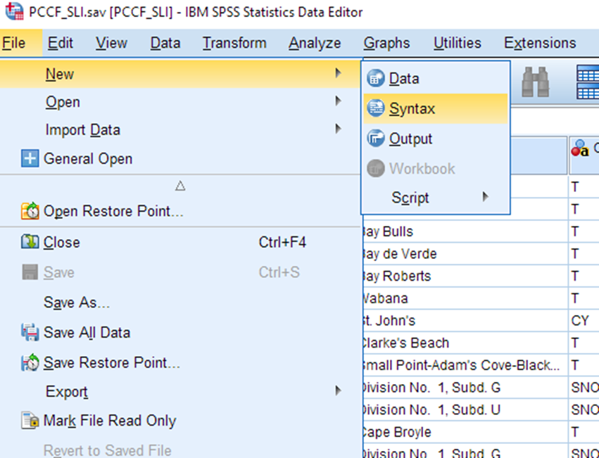
To work with SPSS syntax, first open a new Syntax editor by selecting File > New > Syntax.

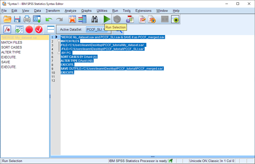
The file PCCF_SLI.sav is open in SPSS Statistics Data Editor. In the toolbar, File is selected. From the drop-down menu, New is selected, followed by Syntax.

A new window opens, probably called Syntax1. This is a window that allows you to type and run SPSS syntax (lines of code). In the white area on the right, type or copy-paste the following lines of code (replace the file path indicated in red text with the file path to wherever you have saved these files:

* SORT My_dataset.sav by PC.

GET FILE ='C:\My_dataset.sav'. 
SORT CASES BY PC.
SAVE OUTFILE='C:\My_dataset.sav'.
EXECUTE.

* SORT PCCF_SLI.sav by PC.
GET FILE ='C:\PCCF_SLI.sav'. 
SORT CASES BY PC.
SAVE OUTFILE='C:\PCCF_SLI.sav'.
EXECUTE.

* MERGE My_dataset.sav and PCCF_SLI.sav & KEEP only the rows in My_dataset.sav & SAVE it as PCCF_merged.sav.

MATCH FILES 
/TABLE='C:\My_dataset.sav'/IN=myresearchdata
/FILE='C:\PCCF_SLI.sav'
/BY PC. 
SELECT IF myresearchdata.
EXECUTE.
DELETE VARIABLES myresearchdata.
EXECUTE.
SAVE OUTFILE='C:\PCCF_merged.sav'
EXECUTE.

After the text has been entered, select all the text and click on the green triangle.

A pop-up titled: Syntax 1 - IBM SPSS Statistics Editor. On the left is a text box. All text is selected. In the toolbar the cursor highlights a green triangle button that will run the selection.

Technique: Quantitative Data Analysis | Tools: R, SAS, SPSS | Data Format: Microdata
Date Created: 2023-06-06 Updated: 2023-07-13