3. Polygon Features

Let’s move on to polygon features. The spatial dataset we will use for polygon features is the City of Toronto’s neighbourhood boundaries shape file. In the section, we will import and map the Toronto neighbourhood boundaries dataset. We will also import the Toronto cultural hot spots point features dataset to combine it with the neighbourhood dataset later in this tutorial.

The Toronto neighbourhoods dataset is called Neighbourhoods - 4326.shp. To import this spatial dataset, we can use the read_sf() function. And we save it as neighbourhoods_sf.

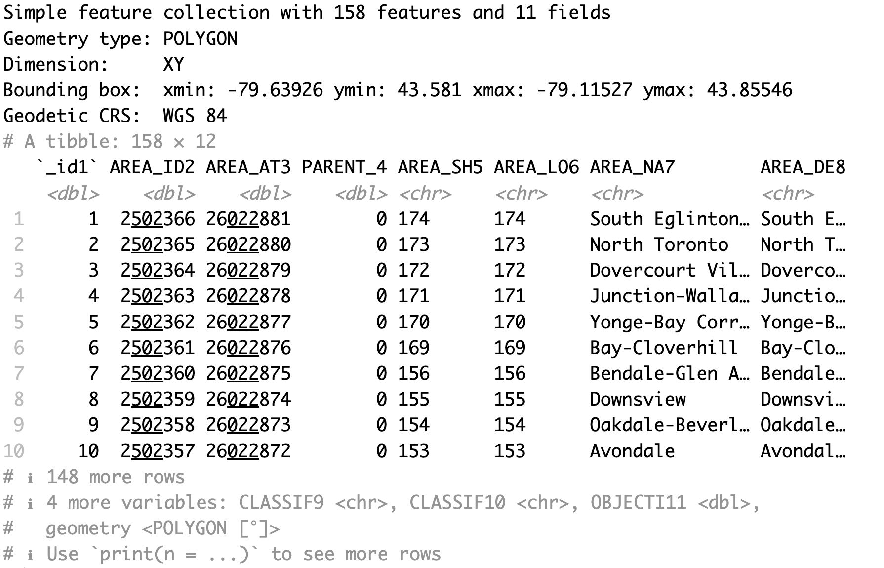
When we run neighbourhoods_sf by itself, we can see that it is a simple features object with 158 polygons or neighbourhoods and 11 fields or variables.

# 3. Polygon Features
# Import Toronto neighbourhoods
neighbourhoods_sf <- read_sf('Neighbourhoods - 4326.shp')
neighbourhoods_sf

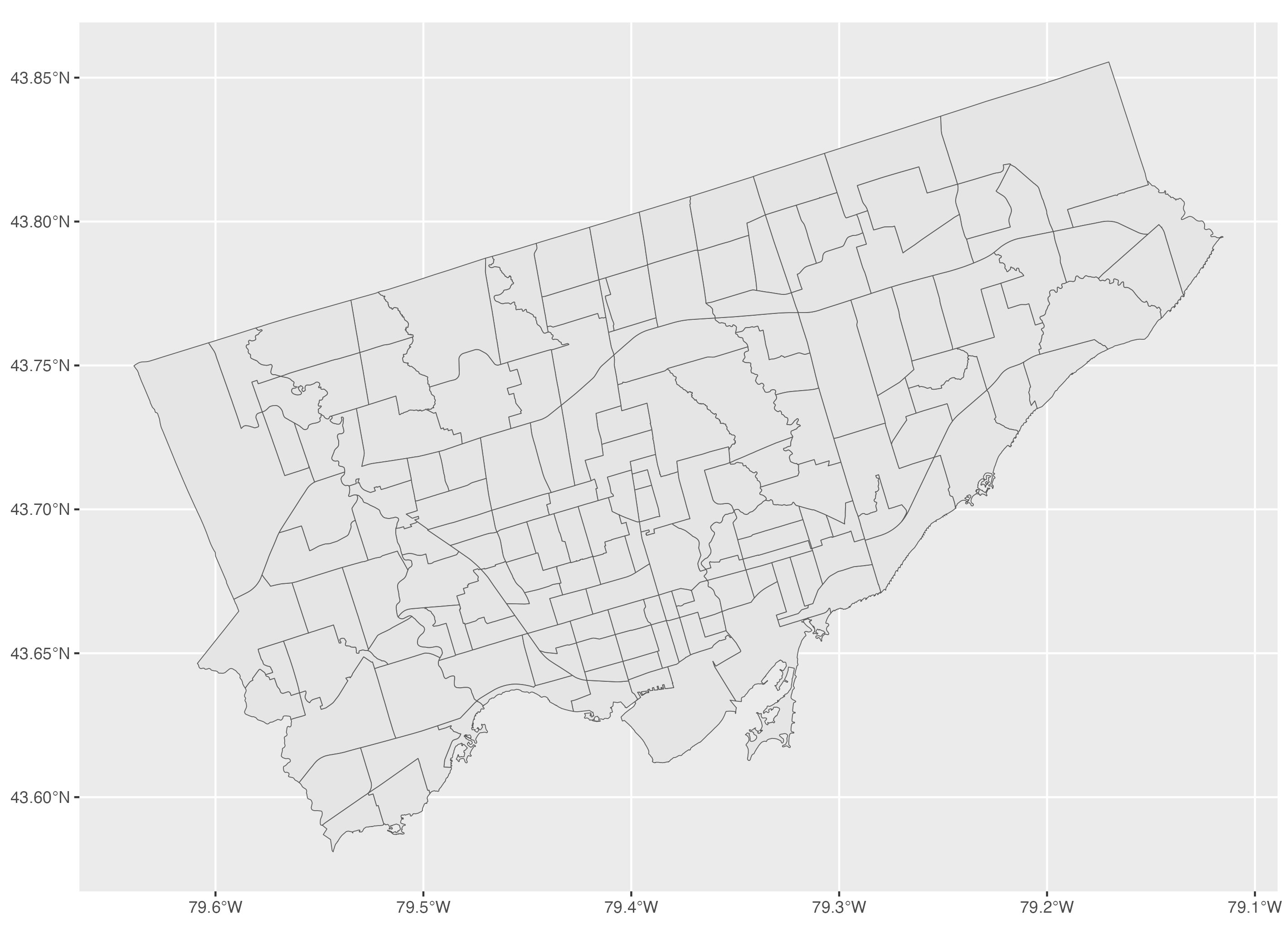
To make a basic map of a polygon features spatial dataset using ggplot2, we use the same approach as we did with point features and line features. We initialize the plot area using the ggplot() function then we specify the neighbourhoods sf object using the geom_sf() function.

# Map Toronto neighbourhoods
ggplot() + geom_sf(data=neighbourhoods_sf)

We will also import the Toronto cultural hot spots dataset. This dataset is called points-of-interest - 4326.shp. We will combine this dataset with the neighbourhoods dataset in section 5. To import this spatial dataset, we can use the read_sf() function. And we save it as culturalhotspots_sf.

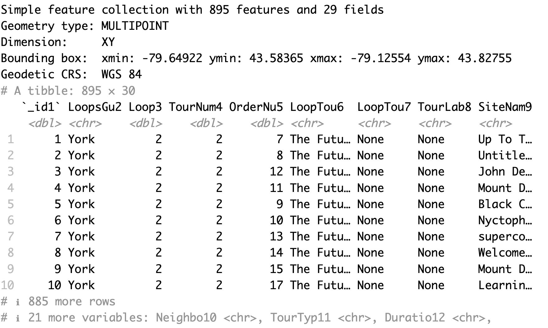
When we run culturalhotspots_sf by itself, we can see that it is a simple features object with 895 point features or hot spots and 29 fields or variables.

# Additional data for Toronto neighbourhoods: Cultural Hot Spots (point features)
culturalhotspots_sf <- read_sf('points-of-interest - 4326.shp')
culturalhotspots_sf

Technique: Quantitative Data Analysis, Mapping, Spatial Analysis | Tools: R | Data Format: Microdata