5. Spatial Analysis

In this section, we will cover running common spatial analyses. We will calculate the length of line features, the distance between features, the nearest feature, and the number of points in a polygon.

First, to calculate the length of line features such as subway lines, we can use the st_length() function and add the subway lines spatial dataset inside. This gives us a list of 4 values which are the lengths of the 4 subway lines in metres.

# 5. Spatial Analysis
## 5.1 Length of Features
# Length of subway lines
st_length(subway_lines_sf)

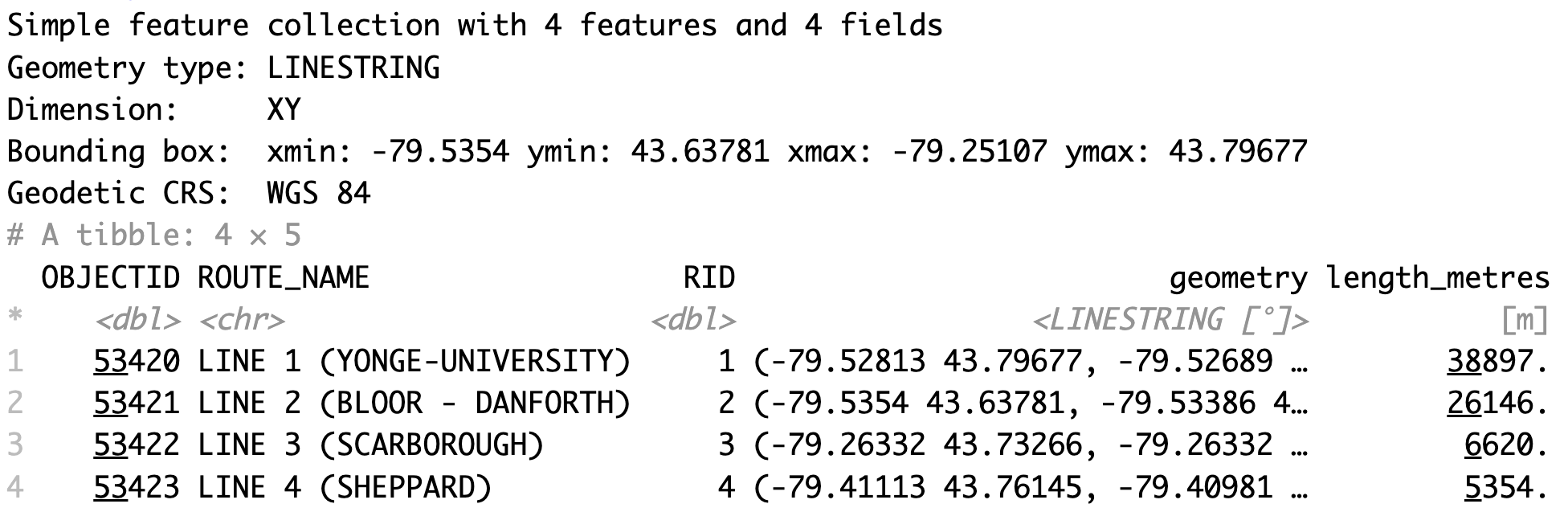
We can store these lengths of subway lines as a new field or variable in the subway lines sf dataset as follows. We start with the subway lines sf object, then we type the name of the new field after a dollar sign, then we assign it the result of the st_length() function with the subway_lines_sf dataset.

Now, when we run the subway_lines_sf dataset, we have 4 fields instead of 3. And you can see the length_metres field is the last column or variable in this dataset.

# Store length as a new variable
subway_lines_sf$length_metres <-st_length(subway_lines_sf)
subway_lines_sf

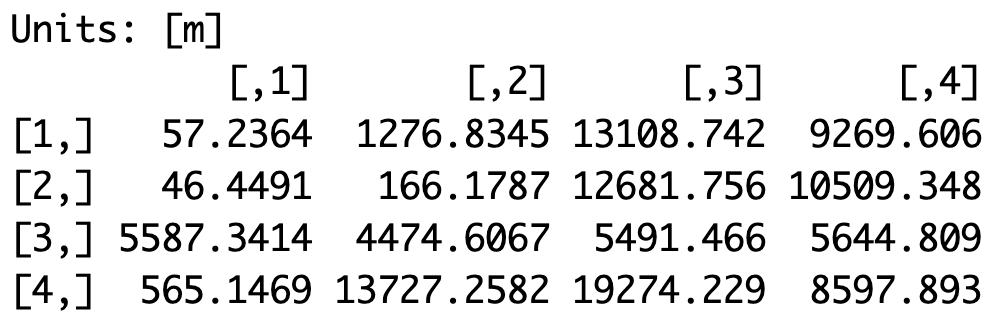
Next, we will calculate the distance between different features. We will start with the distance between point features and line features. To calculate the distance between museums and subway lines, we can use the st_distance() function. Inside this function, we enter the museum and subway lines spatial datasets. This gives us a matrix of distances between each of the 4 museums and each of the 4 subway lines in units of metres. The museums are represented by the rows and the subway lines are represented by the columns.

## 5.2 Distance Between Features: Points vs Lines
# Distance between museums and subway lines
st_distance(museums_sf, subway_lines_sf)

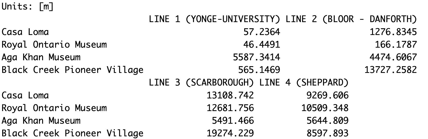
We can save this matrix as a dataset or data frame as follows. First, we convert the matrix of distances using the data.frame() function then we store it as a dataset called dist_table.

Then we rename the rows of dist_table with the names of the museums using the names field from the museums_sf dataset. We also rename the columns with the route names of the subway lines using the route name field from the subway_lines_sf dataset.

Lastly, when we print the dist_table dataset, we can see the dataset of distances with row names and column names.

# Store values in data frame
dist_table <- data.frame(st_distance(museums_sf, subway_lines_sf))
# Assign names to rows and columns
rownames(dist_table) <- museums_sf$names
colnames(dist_table) <- subway_lines_sf$ROUTE_NAME
dist_table

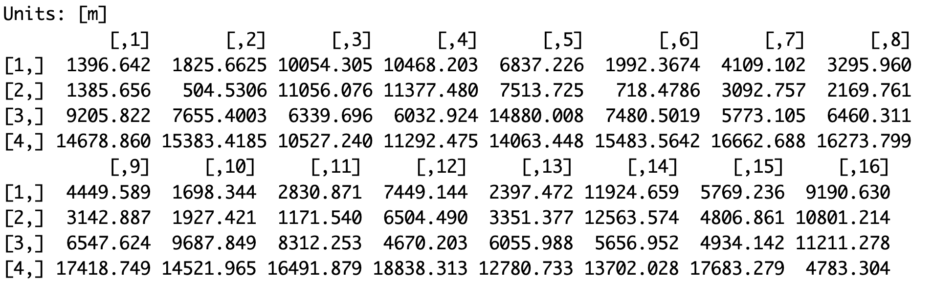
Next, we will calculate the distance between two sets of point features: the distance between museums and subway stations. Again, we use the st_distance() function to calculate the distance between the museums and the subway stations sf datasets. This gives us a matrix of distances in units of metres. Again here, the rows are represented by the museums and the columns are represented by the subway stations.

## 5.3 Distance Between Features: Points vs Points
# Distance between museums and subway stations
st_distance(museums_sf, subway_stations_sf)

Next, we want to find the nearest subway station to each museum and store it in the museums dataset. To find the nearest subway station, we can use the st_nearest_feature() function. We enter the museums sf dataset first then we enter the subway stations sf dataset. This gives us the index of the nearest subway station for each museum.

## 5.4 Nearest Feature
# Find the nearest subway station index for each museum
st_nearest_feature(museums_sf, subway_stations_sf)

We can use the indices to identify the subway station names as follows. We type the name variable from the subway_stations_sf dataset. Then inside square brackets, we add the code above with the subway station indices. This gives us the four names subway stations associated with the four indices above.

# Use index to identify subway station name
subway_stations_sf$Name[st_nearest_feature(museums_sf, subway_stations_sf)]

To save the nearest station names in the museums spatial dataset, we assign the line of code above to a new field or variable that we call nearest_subway_station in the museums sf dataset.

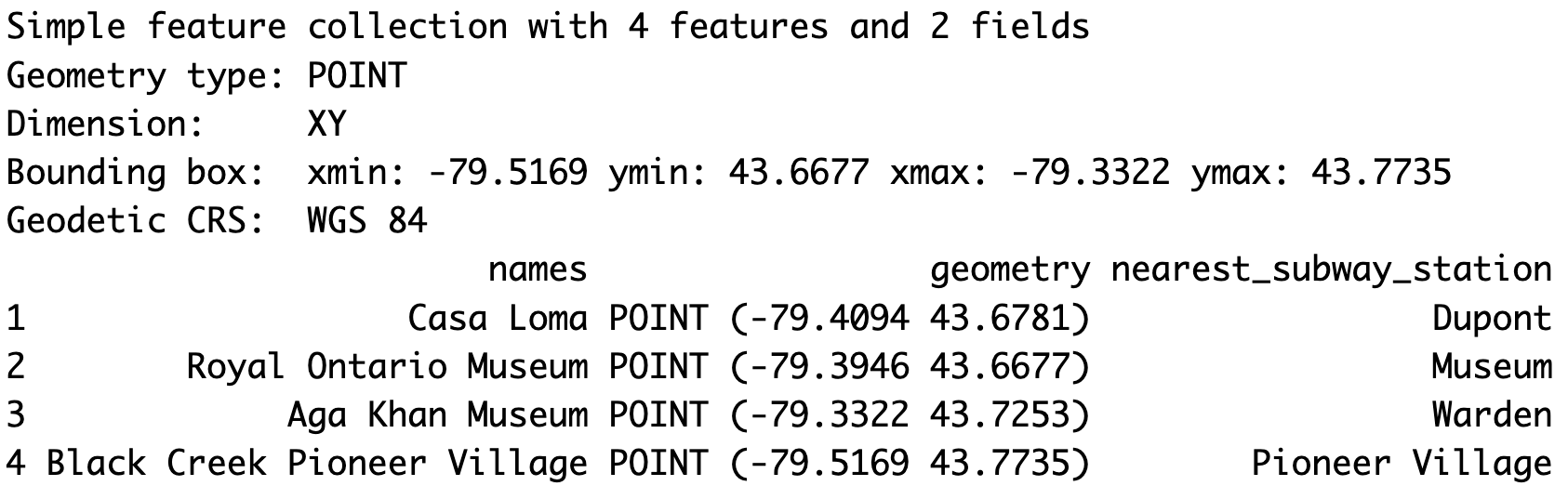
Now, when we run the museums_sf dataset, we can see that it has two fields instead of just one. And the last column is the nearest subway station.

# Save list of nearest stations
museums_sf$nearest_subway_station <- subway_stations_sf$Name[st_nearest_feature(museums_sf, subway_stations_sf)]
museums_sf

Finally, we calculate the number of points in a polygon. In this tutorial, we will calculate the number of cultural hot spots in each Toronto neighbourhood. To do this, first we use the st_intersects() function with the neighbourhoods and the cultural hot spots spatial datasets to identify the cultural hot spots that intersect with each neighbourhood. This code gives us, for each neighbourhood, the list of cultural hot spots that intersect with it.

Then to count the number of cultural hot spots in each neighbourhood, we use the lengths() function around the st_intersects() function. As you can see below, this gives us a list of the number of cultural hot spots for each neighbourhood.

## 5.5 Number of points in polygon
# Number of cultural hot spots in each neighbourhood
lengths(st_intersects(neighbourhoods_sf, culturalhotspots_sf))

We save this number as a new field in the neighbourhoods_sf dataset and name it counthotspots. We will use this new field counthotspots in the next section.

# Store number as a new variable
neighbourhoods_sf$counthotspots <- lengths(st_intersects(neighbourhoods_sf, culturalhotspots_sf))

Technique: Quantitative Data Analysis, Mapping, Spatial Analysis | Tools: R | Data Format: Microdata