Loading Data

Data can be added to QGIS from many different sources, including:

• Shapefiles
• Esri geodatabase
• Geopackage
• Spreadsheet
• Databases (PostgreSQL, SpatialLite, and others)
• Image file (raster data)
• Web service (WFS, WMS)

Shapefiles

Shapefiles are one of the most common vector file formats used in GIS.

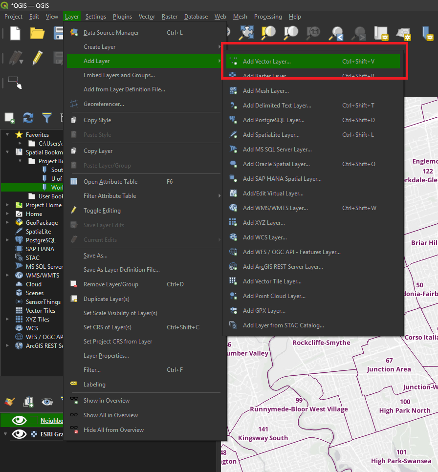
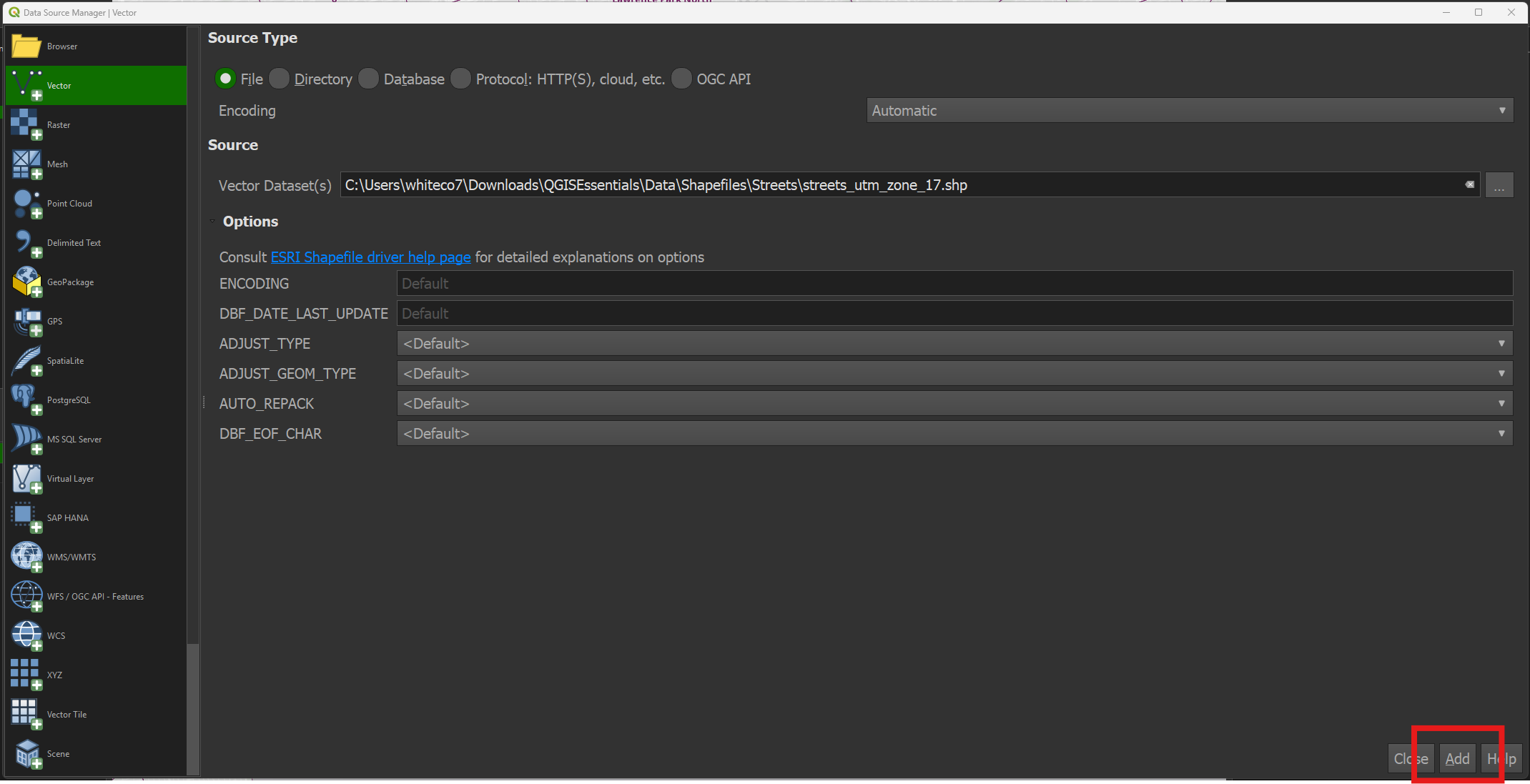
• Select Layer → Add Layer → Add Vector Layer from the menu.

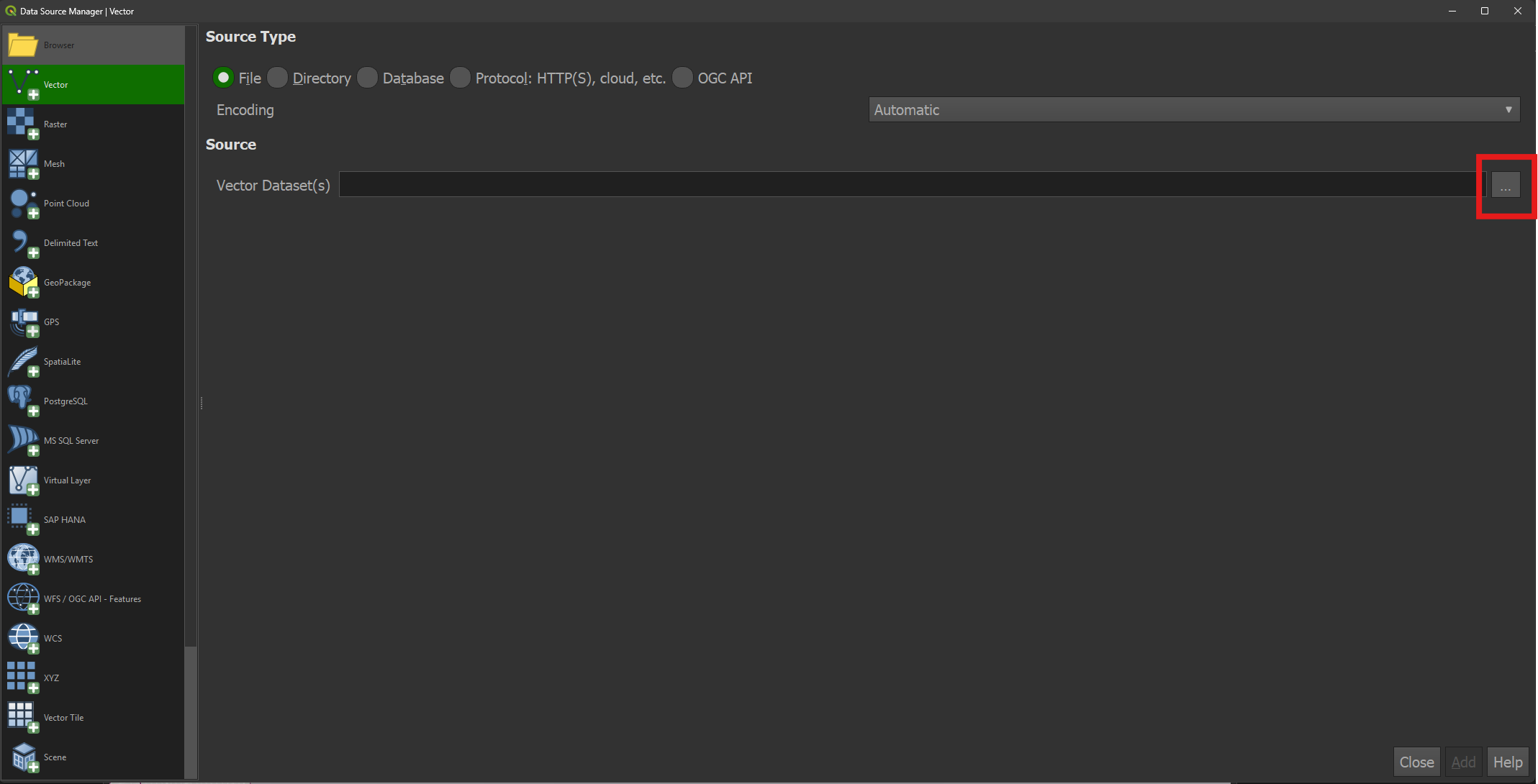
• In the Data Source Manager, click the three dots next to the Vector Datasets(s) box.

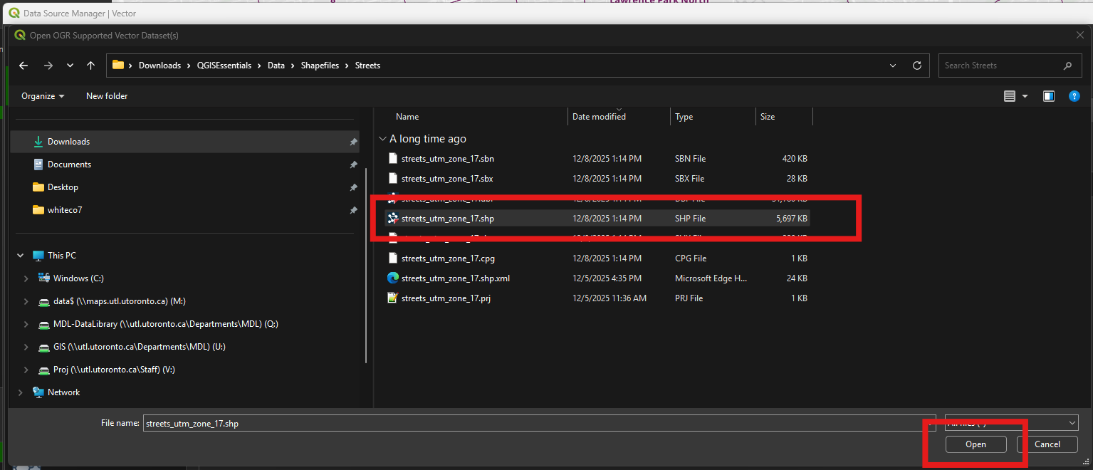
• Browse to the Data → Shapefiles → Streets folder. Select streets_utm_zone_17.shp. Click Open.

• Click Add. Close the Data Source Manager.

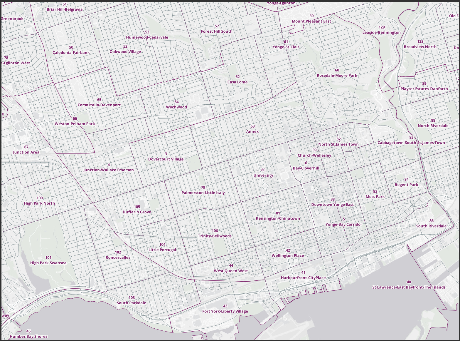
• Result: A new spatial layer, representing Toronto’s street network, has been added to the map. (Note: This dataset was obtained from the City of Toronto’s Open Data website here: https://open.toronto.ca/dataset/toronto-centreline-tcl/)

Spreadsheets

Data can be imported into GIS from spreadsheets (.csv, .xlsx, etc.) Spreadsheets can be automatically transformed into spatial layers if they contain geographic information (coordinates). Spreadsheet data can also be joined to spatial layers based on common attribute values, or converted from written text using a process called geocoding.

Add a spreadsheet containing geographic coordinates

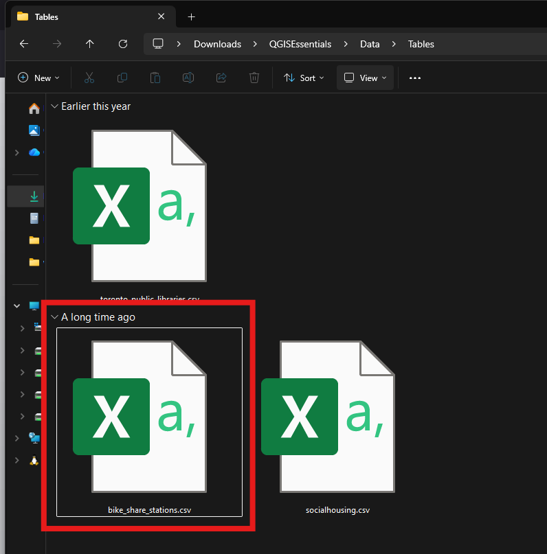
• On your computer, navigate to the Data → Tables folder within the data folder. Double-click bike_share_stations.csv to open it in Excel or other software that can view spreadsheets.

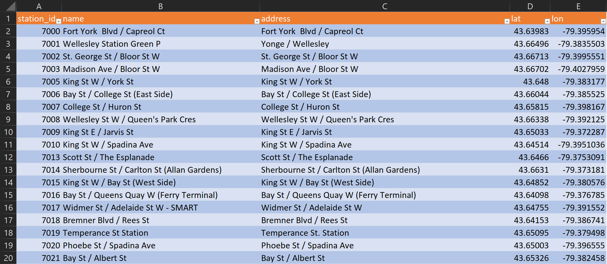
• Note that each bike share station has latitude and longitude coordinates associated with it, in columns called ‘lat’ and ‘lon’, respectively. Close the spreadsheet.

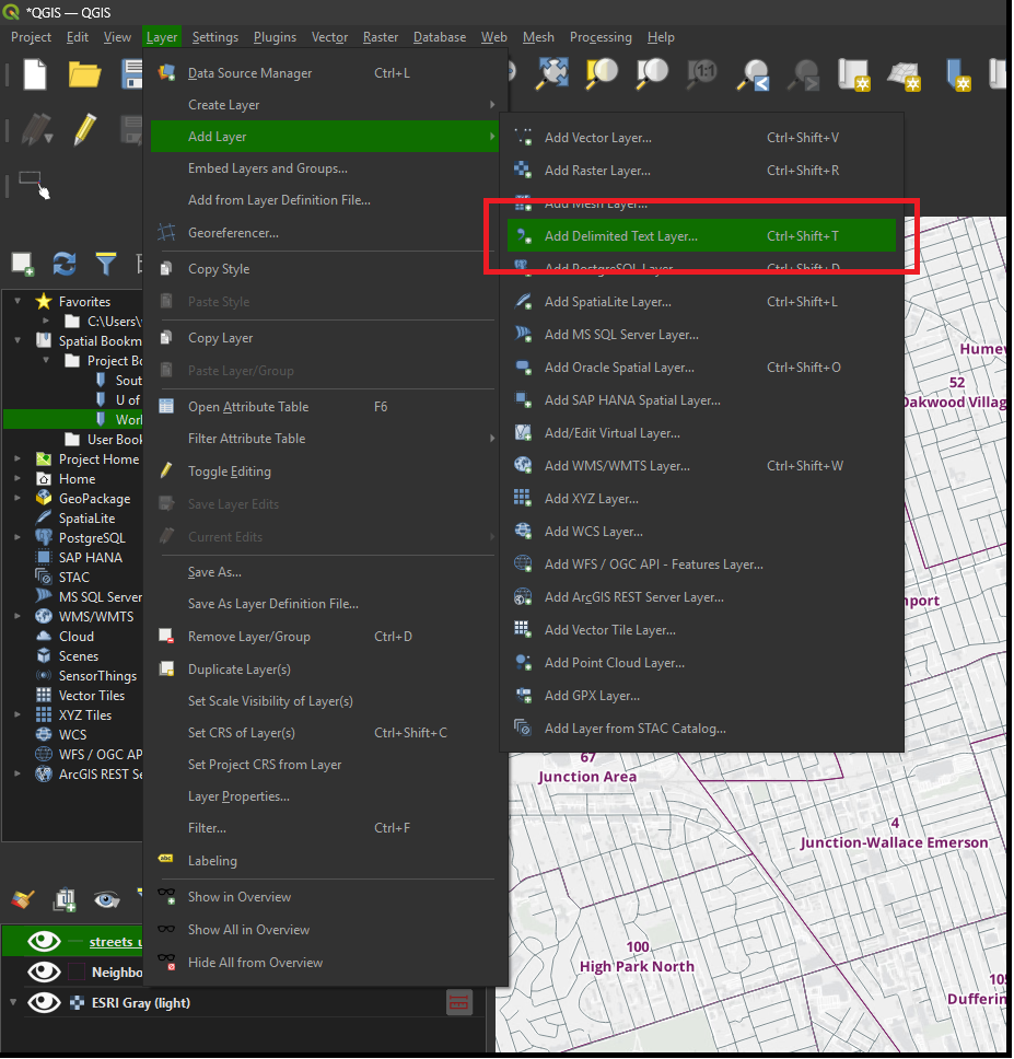
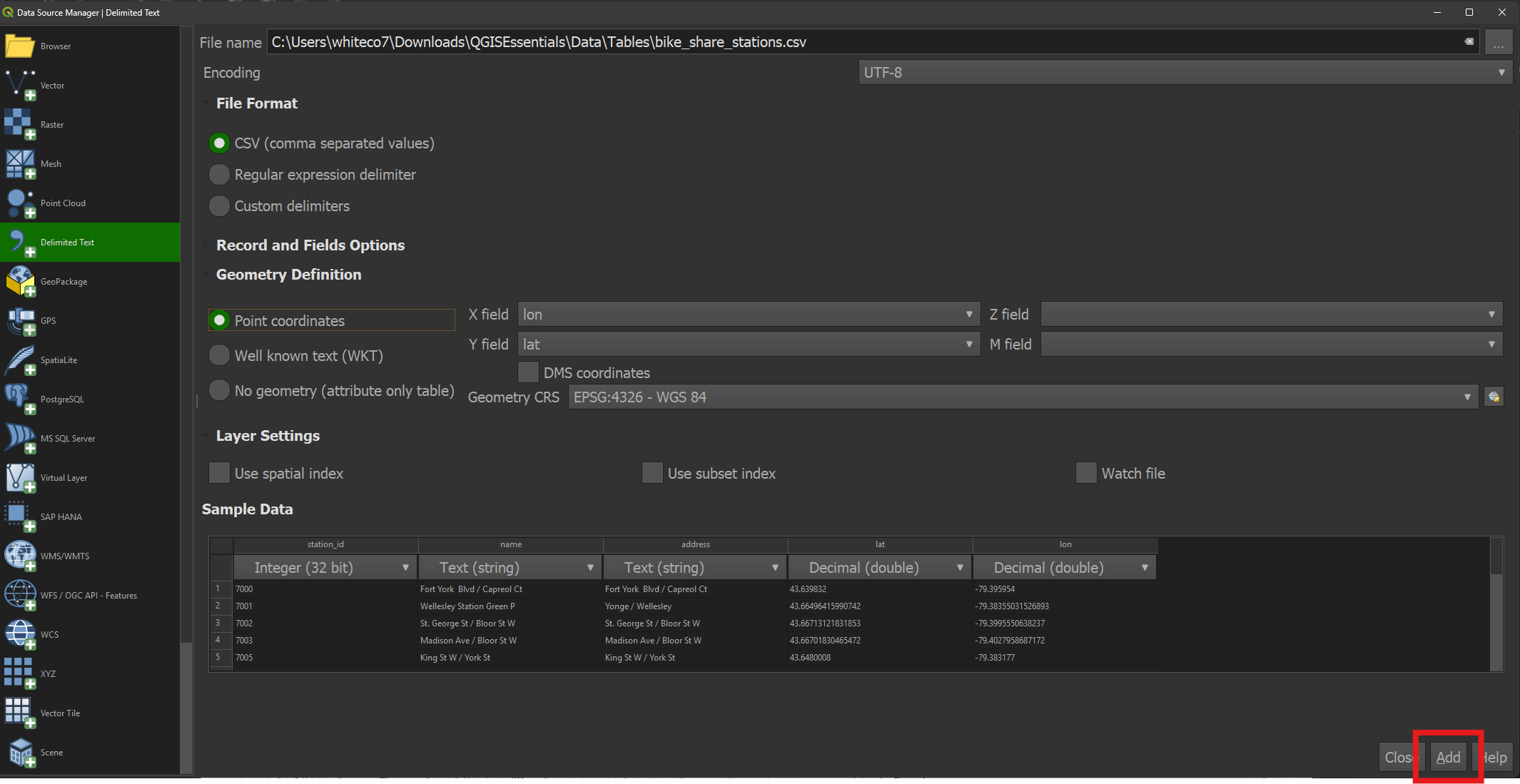
• In QGIS, click Layer → Add Layer → Add Delimited Text Layer.

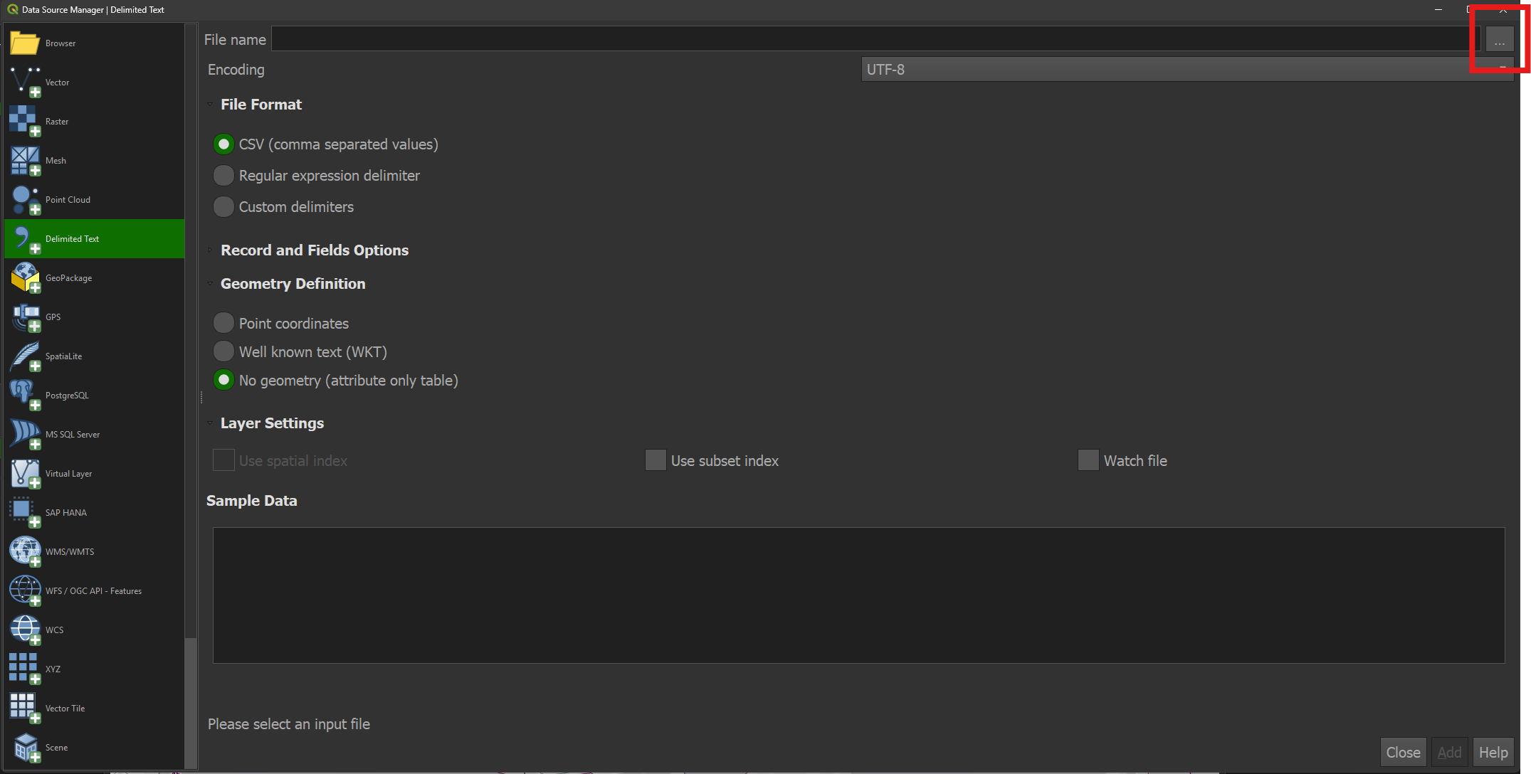
• Click the three dots next to the File name box.

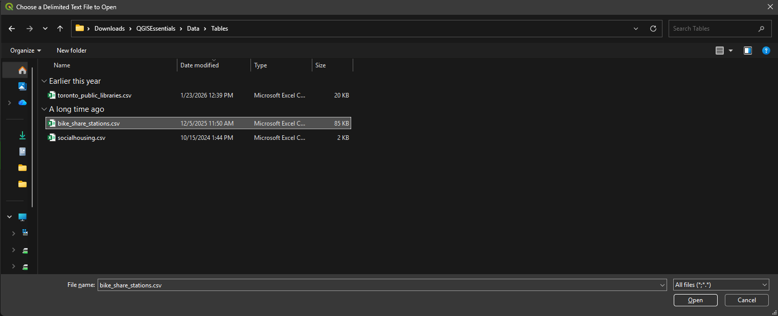
• Navigate to bike_share_stations.csv and click Open.

• Under the Geometry definition heading, click Point coordinates. Make sure lon has been selected for the X field, and lat has been selected for the Y field.

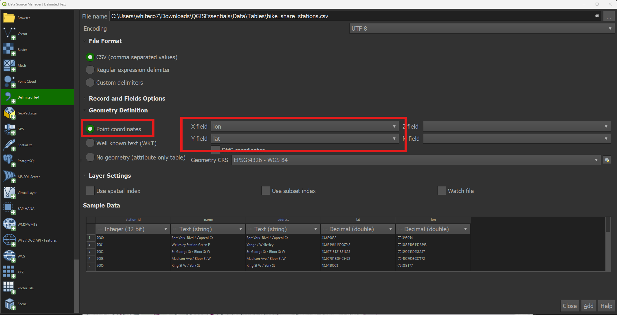
• Click Add. Close the Data Source Manager.

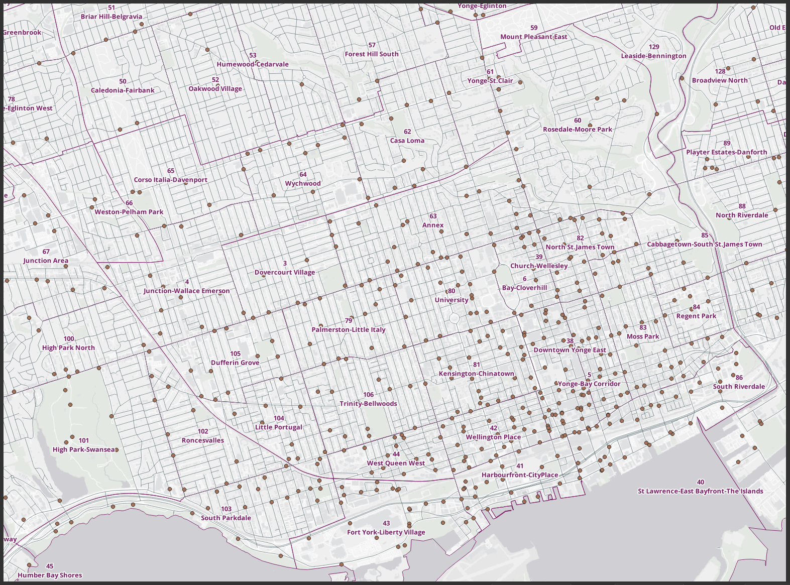
• Result: a point layer showing bike share station locations has been added to the map.

Add data from a spreadsheet with geocoding

Geocoding attempts to match natural language street addresses to a physical location on the earth’s surface.

Example: 130 Saint George Street, Toronto ON M5S 0C2 = Lat: 43.664, Long: -79.399.

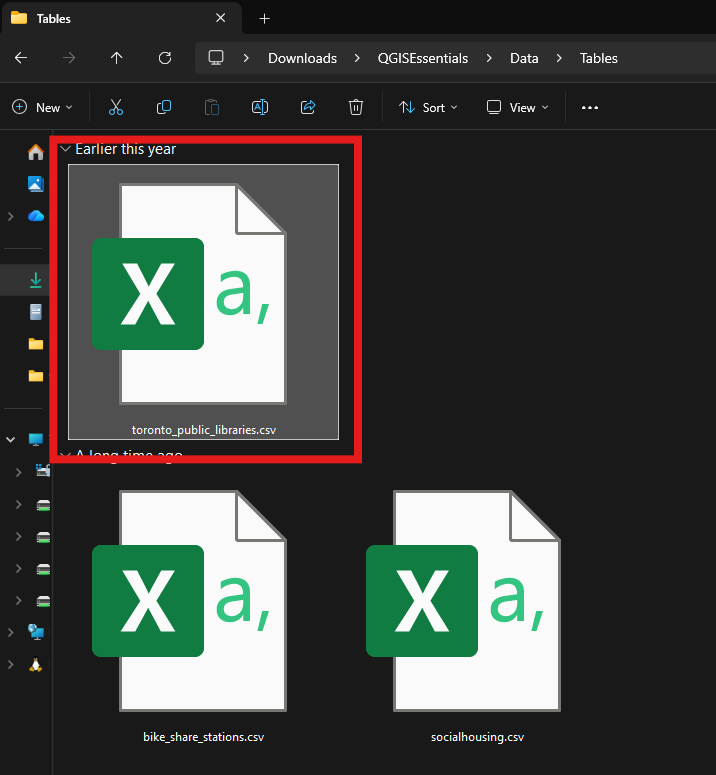
• Navigate to the data folder and open toronto_public_libraries.csv in Excel or another spreadsheet viewer.

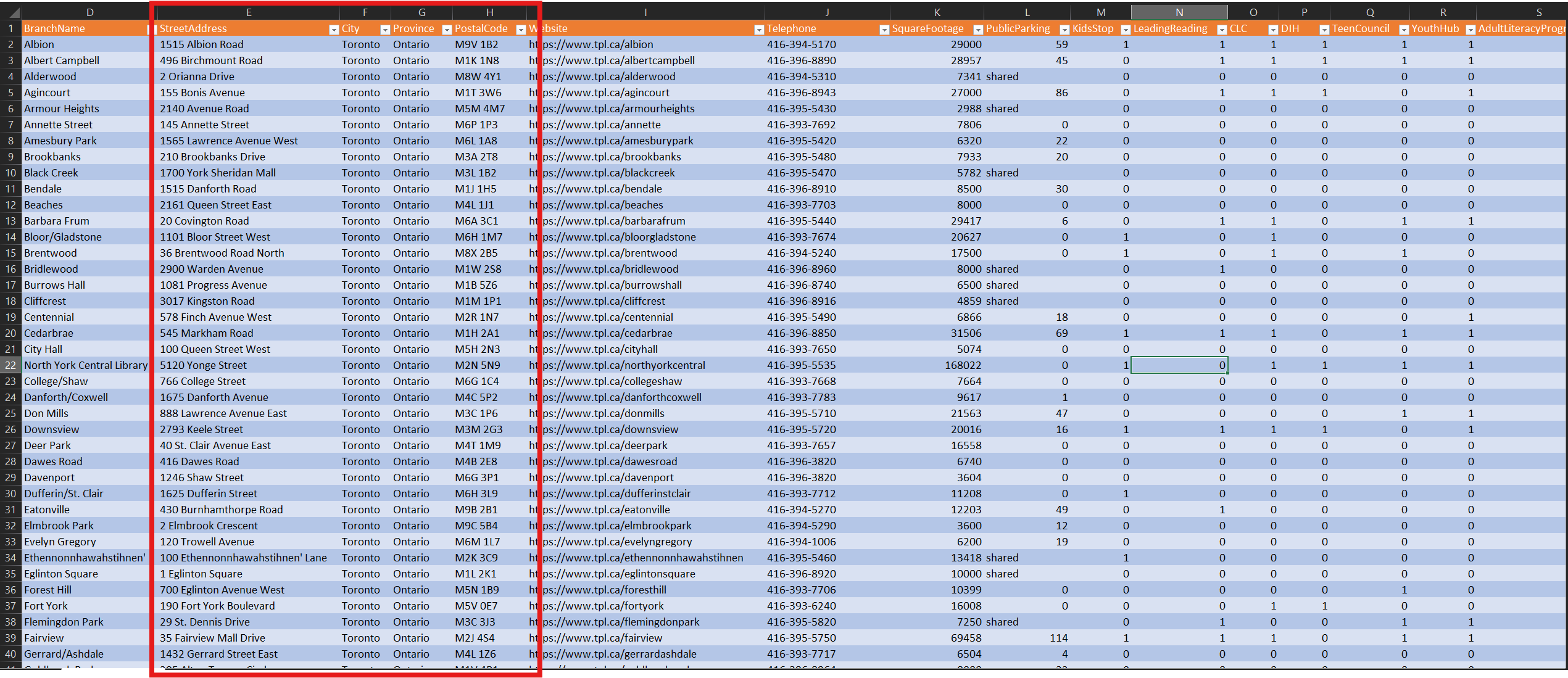
• Note the columns containing street address information. Close the spreadsheet.

• In QGIS, select MMQGIS → Geocode → Geocode CSV with web service. (If you don’t have this option, install the MMQGIS plugin as described in the Plugins section.)

<img src=’/qgis-mapping-spatial-analysis-intro/assets/images/geocode-with-web-service.png’ alt=”MMQGIS - Geocode CSV with web service”” width=’100%’ height=’100%’ />

• Navigate to and select toronto_public_libraries.csv as the Input CSV File.

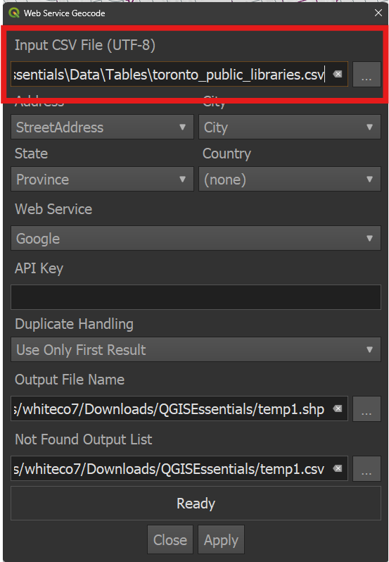
• Select the StreetAddress, City, and Province columns for the Address, City, and State parameters (if QGIS hasn’t already done this automatically).

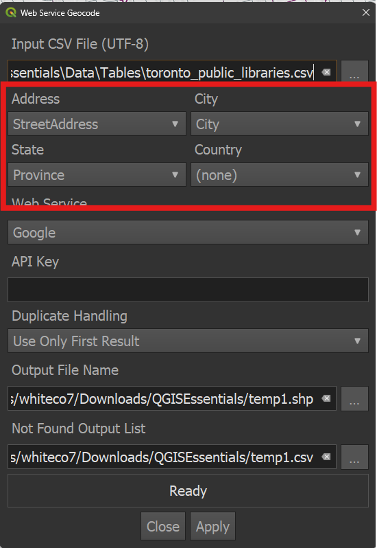
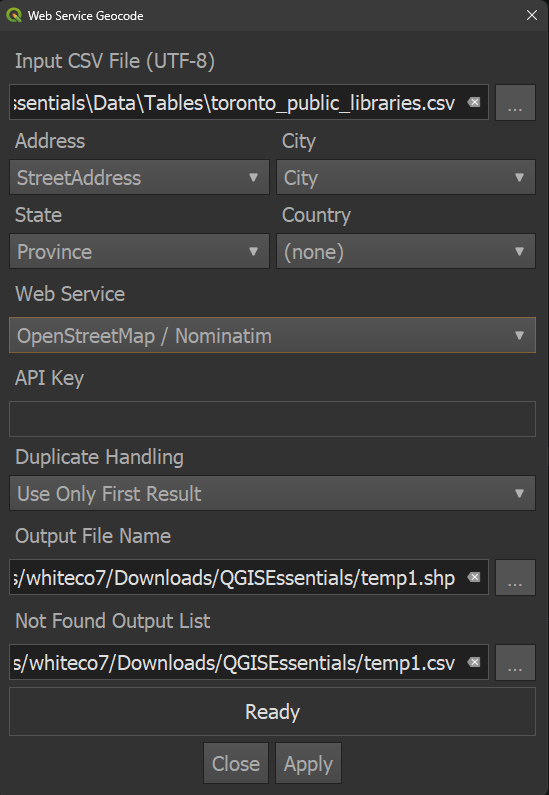
• Choose OpenStreetMap/Nominatim for the Web Service.

• Save the geocoding results in the data folder as library_geocode.shp. Save the Not Found Output Last in the data folder as library_geocode_errors.csv. Click Apply.

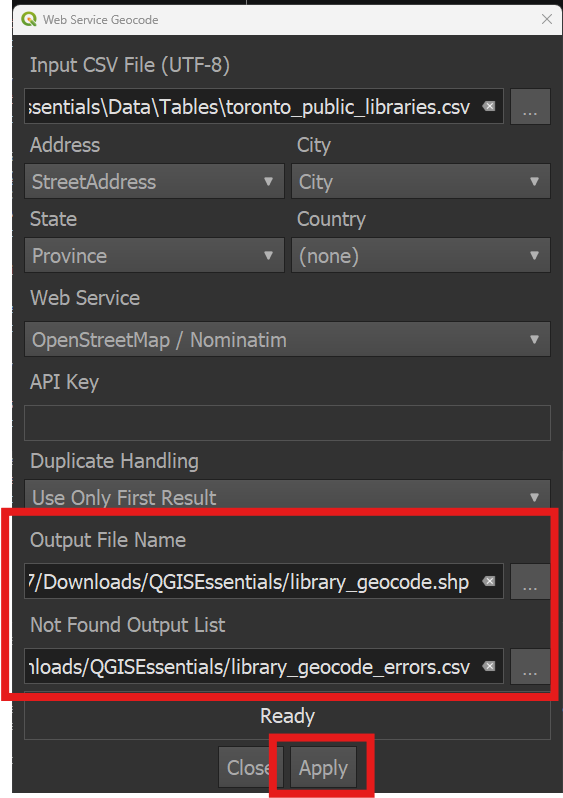
• QGIS may be unresponsive for a few moments while the plugin queries the web service. Once it has completed, however, a results message will be displayed. Click Close.

• Result: a new point layer showing public library locations has been added to the map. The layer’s attribute table contains the information from the csv.

• Records for which the geocoder couldn’t figure out a location are recorded in the library_geocode_errors.csv file.

Attribute joins

Attribute joins append columns from one table (layer) to another, based on a common matching field.

Joining data in this way is very common in GIS and in working with databases.

• Navigate to the Tables folder and open socialhousing.csv. This dataset shows the number of social housing units (including those that are rent geared to income) in Toronto, by neighbourhood. Note that there are 127 total records.

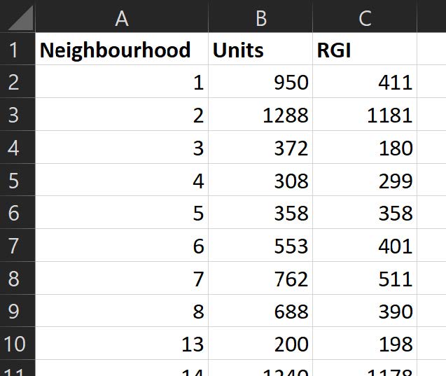
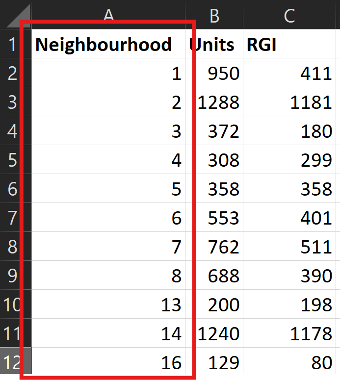
• Each neighbourhood in the spreadsheet is signified by an ID number that the City has designated. This number is stored in the Neighbourhood column.

• The Neighbourhoods polygon layer in QGIS also has this ID number in its attribute table. It is stored in the Neighbourhood ID field.

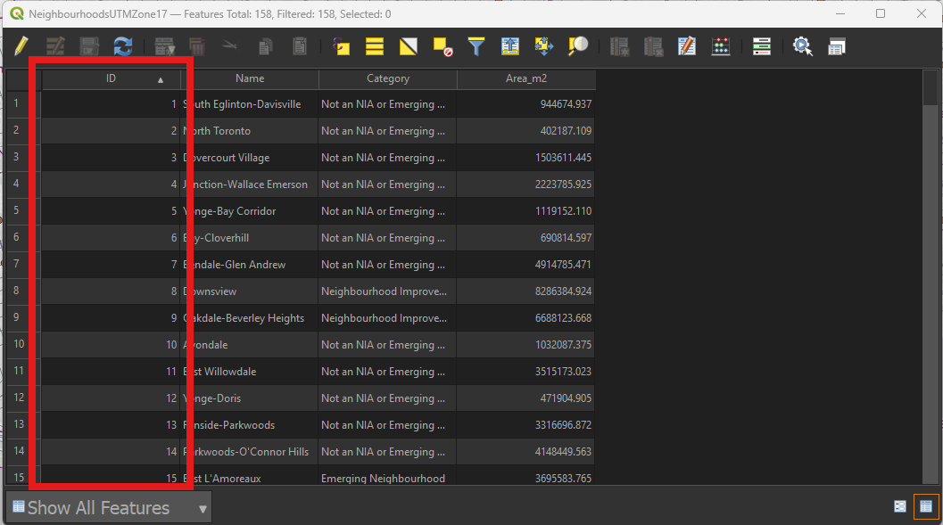
We’ll use a join to attach the spreadsheet data to the polygon layer.

First, we’ll add the CSV to the QGIS project:

• Select Layer → Add Layer → Add Delimited Text Layer.

• Navigate to and select socialhousing.csv. Choose no Geometry (Attribute only table).

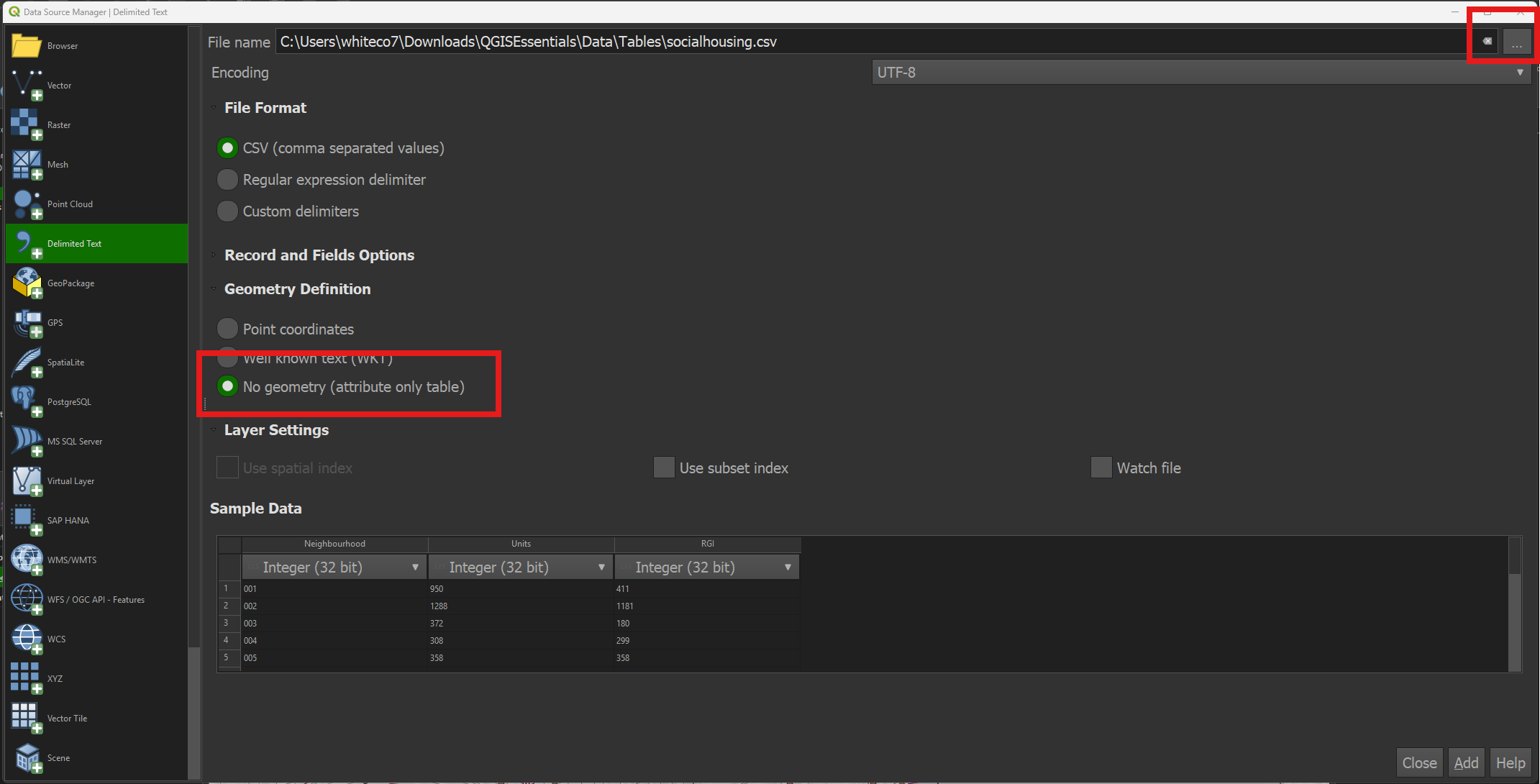
• Click Add. Close the Data Source Manager. The csv will be added to the project as a table. It will be listed in the Layers panel, but nothing will be added to the map.

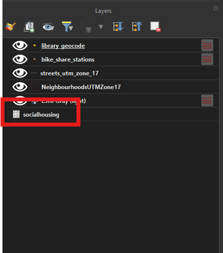
Create the join:

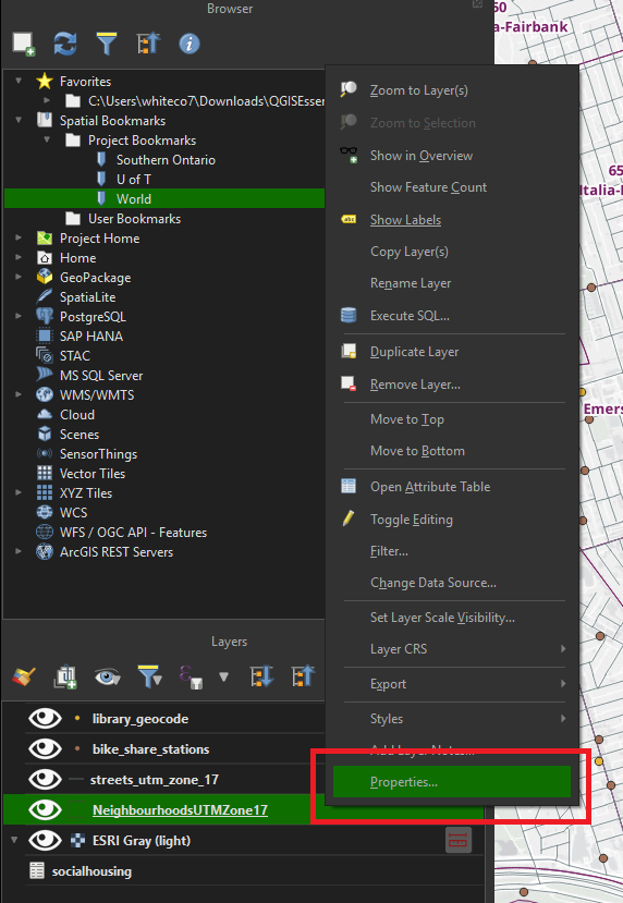
• Right-click (Control-click on Mac) the neighbourhoods layer. Select Properties.

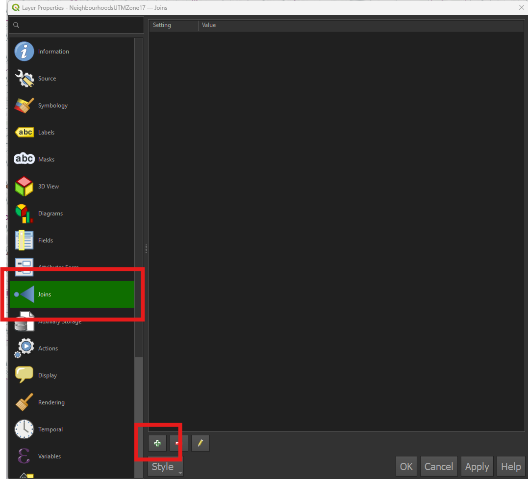
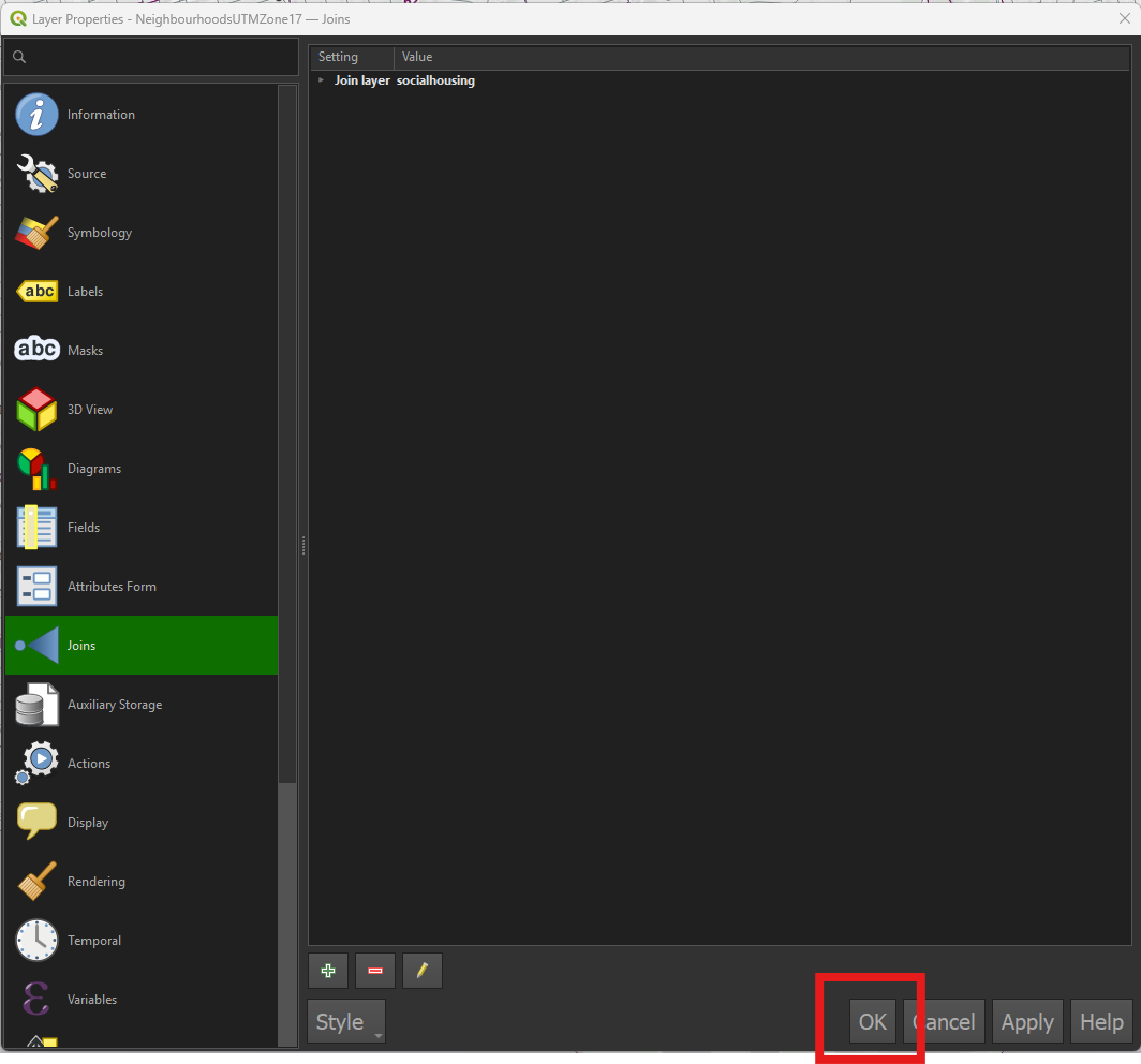
• Click the Joins tab. Click the + (plus sign) button.

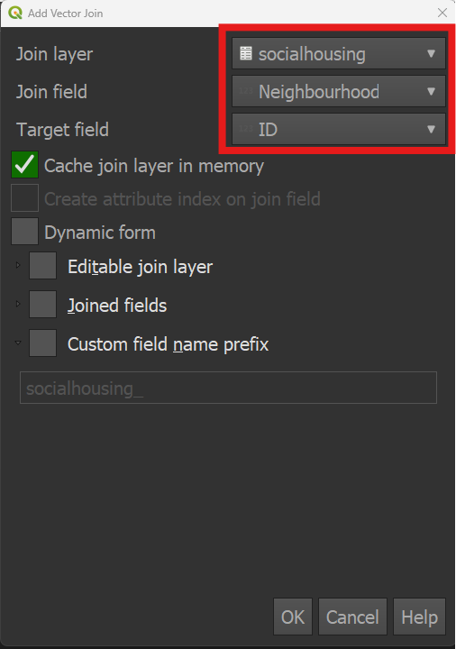
• Choose socialhousing as the Join layer, Neighbourhood as the Join field and ID as the Target field. Click OK.

• Note that the join is now listed in the layer properties. Click OK to close the layer properties window.

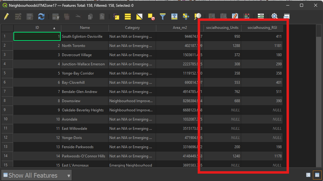
• Open the attribute table of the neighbourhoods layer. The social housing columns are now part of this table.