Geoprocessing

Geoprocessing allows us to transform and analyze spatial data.

Geoprocessing tools in QGIS typically take one or more layers as an input and produce a new layer as an output.

QGIS includes many geoprocessing tools. More can be added via plugins.

Filtering data

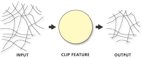
Image source: Wikimedia Commons. CC-BY-SA 4.0.

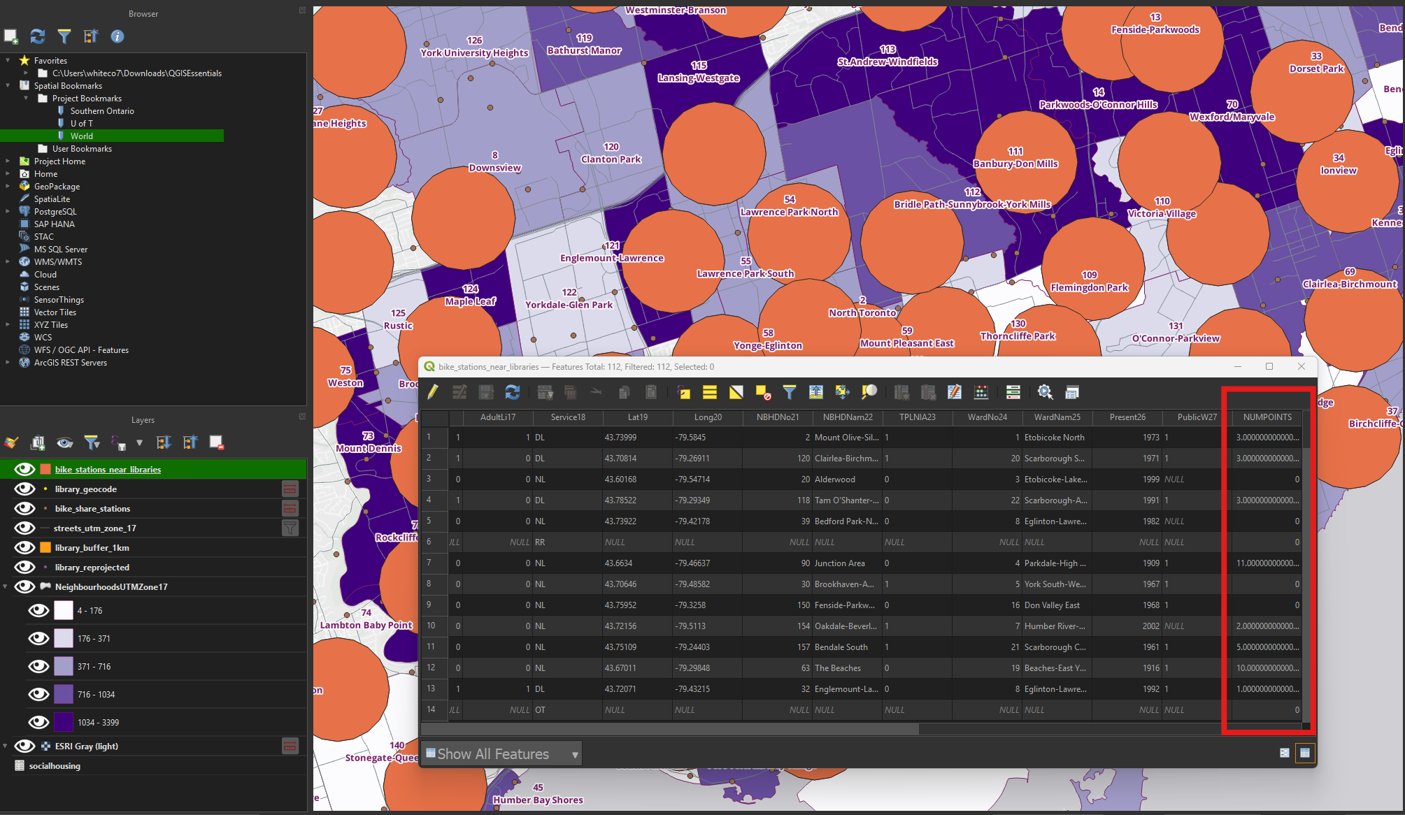
We’ll use geoprocessing to analyze areas around each public library location.

To prepare for this, we will need to reproject the libraries layer. (This is because the spreadsheet data used latitude and longitude, which is an angular unit of measurement. We need to change this to a linear unit - e.g., metres.)

Reprojecting data

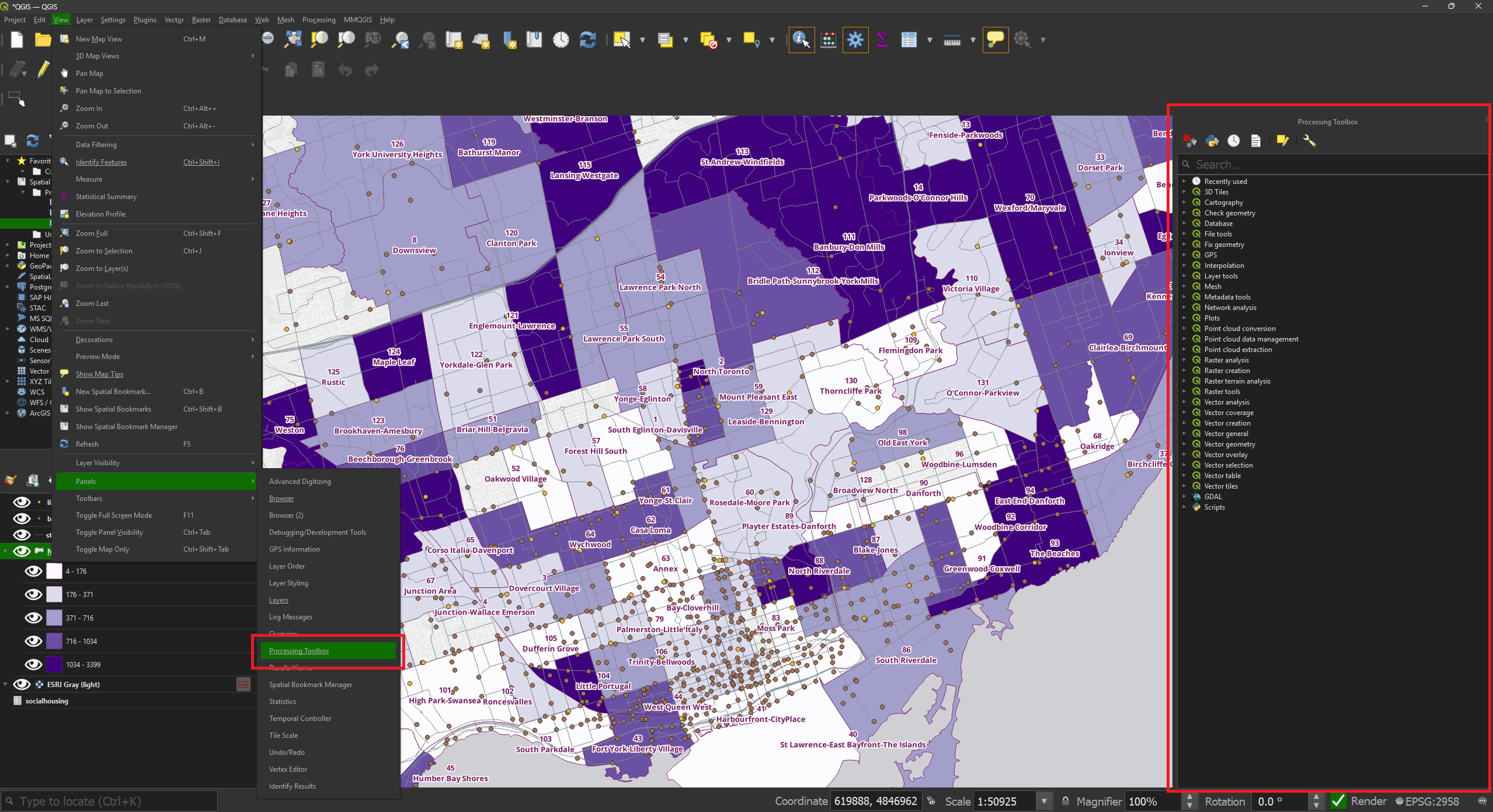
• Open the Processing Panel (View → Panels → Processing Toolbox) if it’s not already open.

QGIS processing toolbox

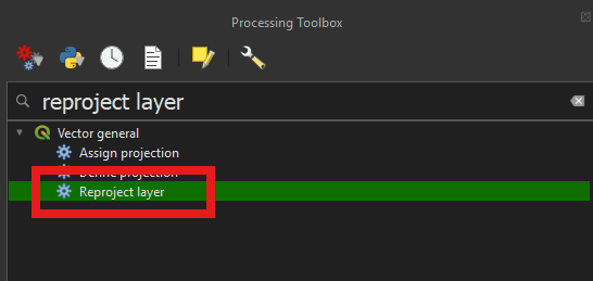
• Search for reproject layer. Double-click the Vector general → Reproject layer result to open the tool.

Processing toolbox → Vector general → Reproject layer

• For the Input layer, select the libraries layer from the dropdown.

Input layer = libraries

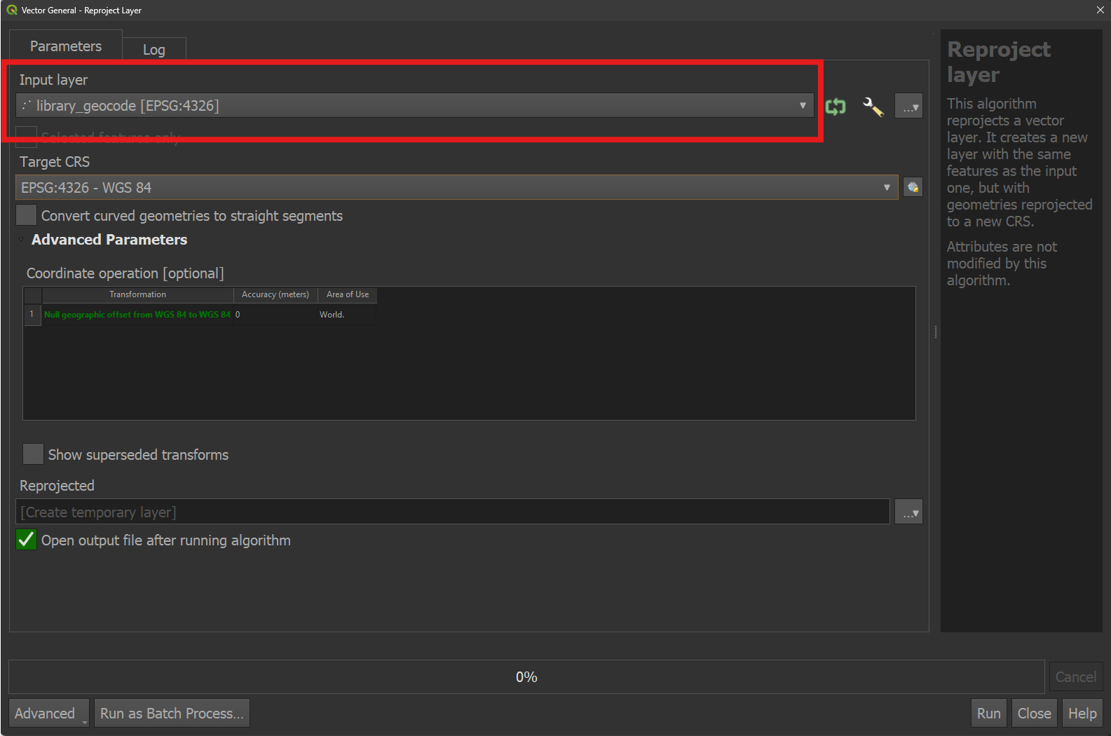
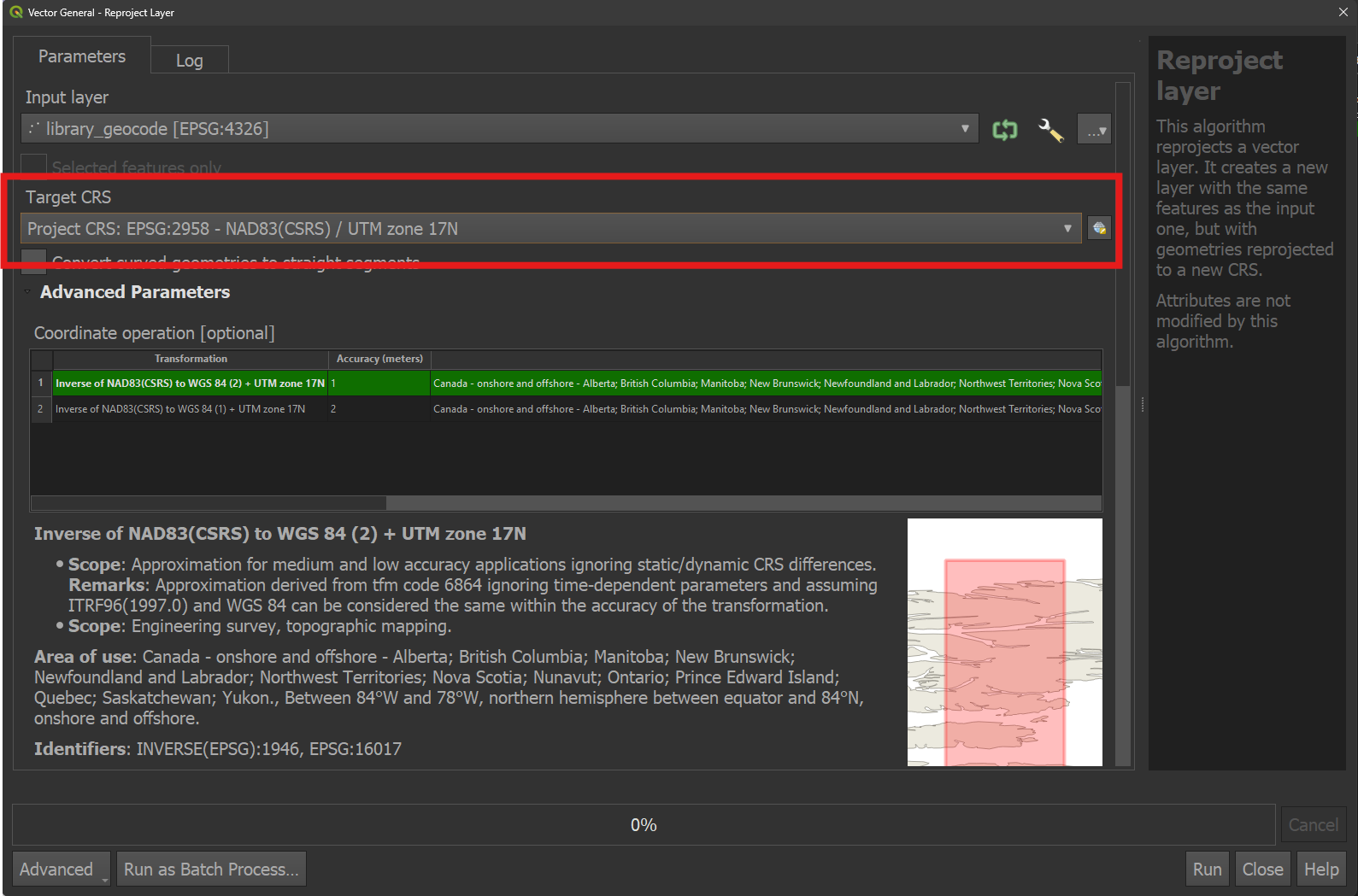
• For the Target CRS, choose Project CRS: EPSG:2958 - NAD83(CSRS) / UTM Zone 17N from the dropdown.

Target CRS = Project CRS

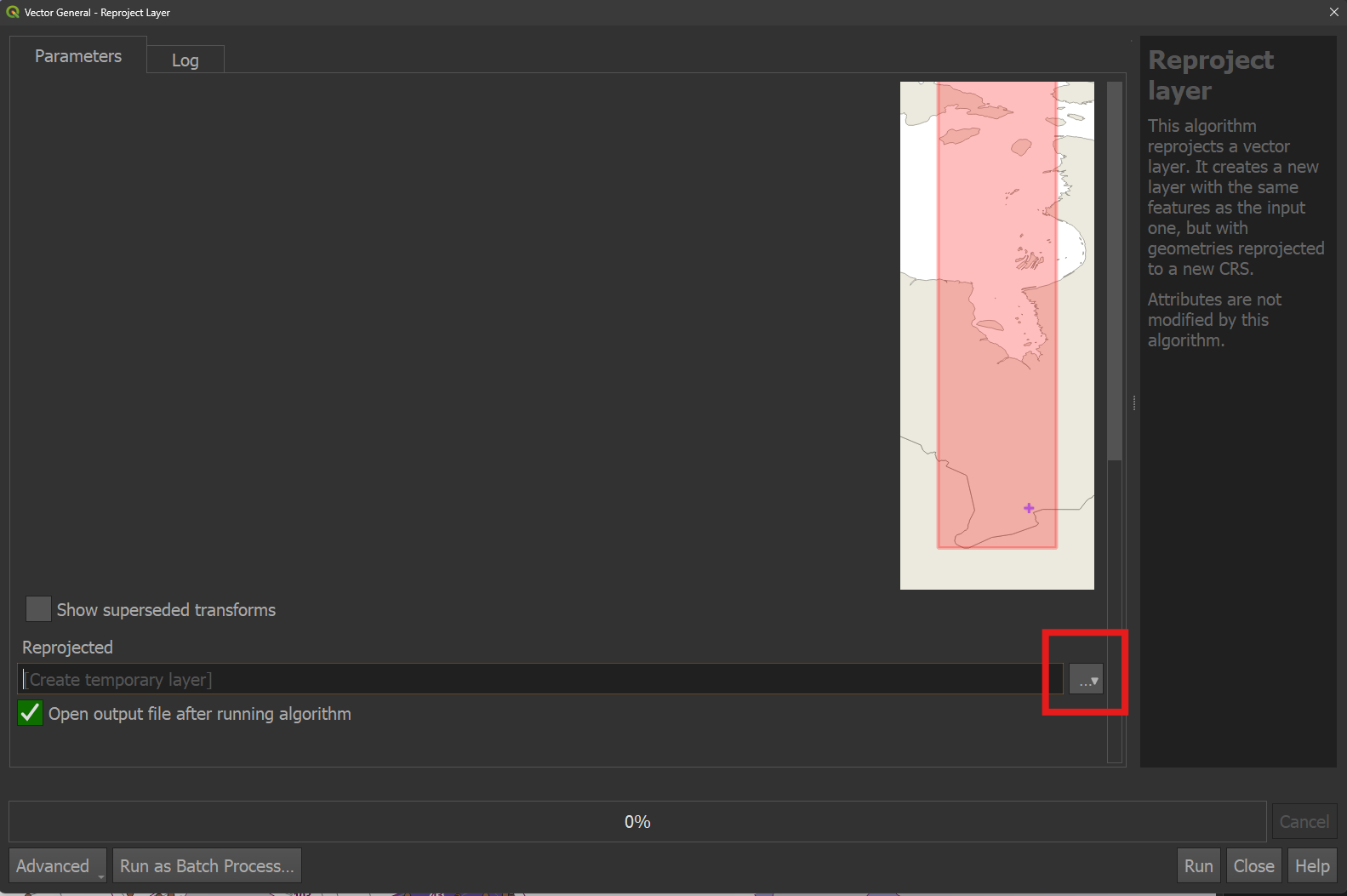
Save the output as a shapefile:

• Click the three dots next to the Reprojected box and choose Save to File.

Saving output to file

• Navigate to the data folder and save the output as library_projected.shp. Click Run.

Run the tool

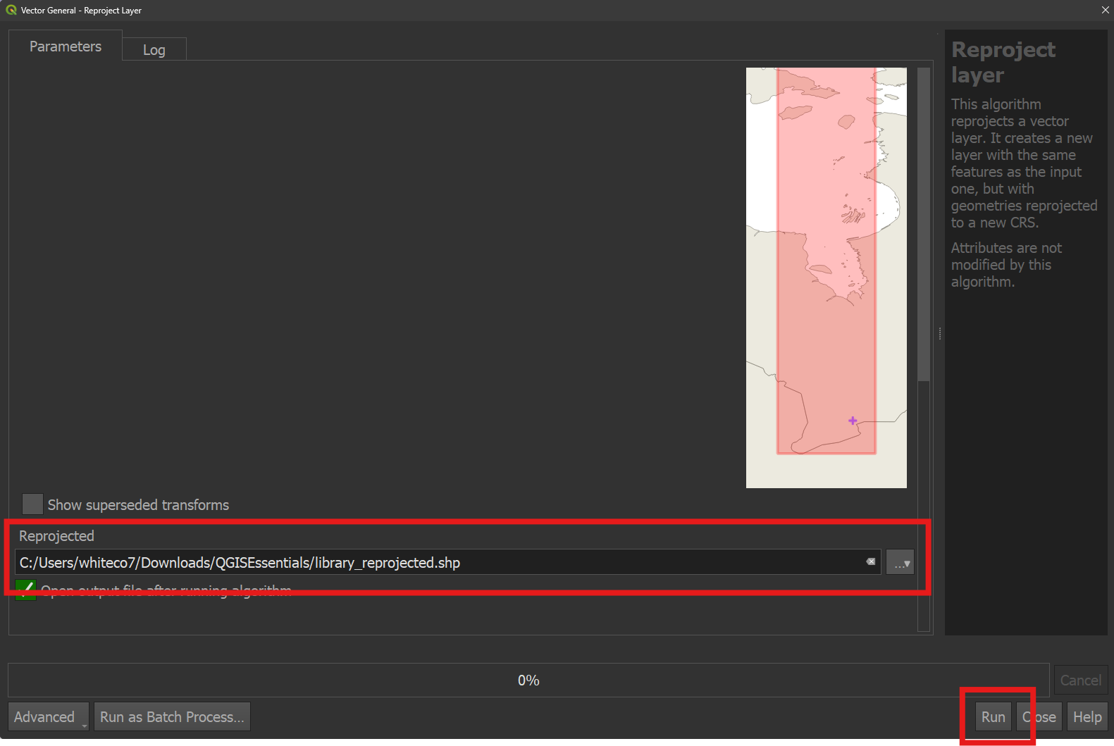
The result is a new version of the libraries layer that uses a different coordinate reference system. (Note that you can display the underlying CRS by hovering over the layer name).

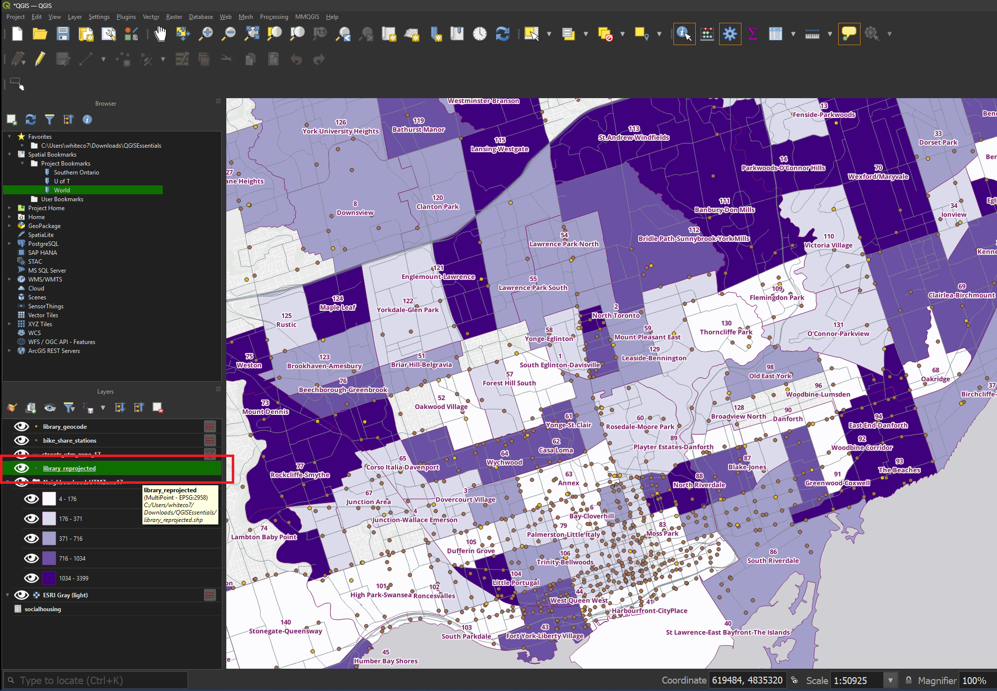
Reprojected output layer in map canvas

Buffering features

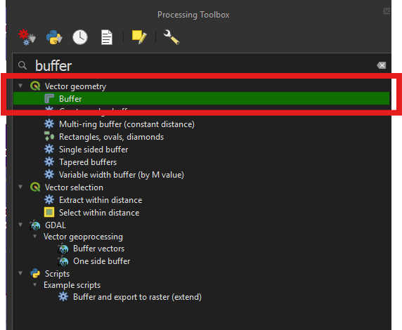
• Search for Buffer in the Processing Toolbox. Double-click the Vector Geometry → Buffer result to open the tool.

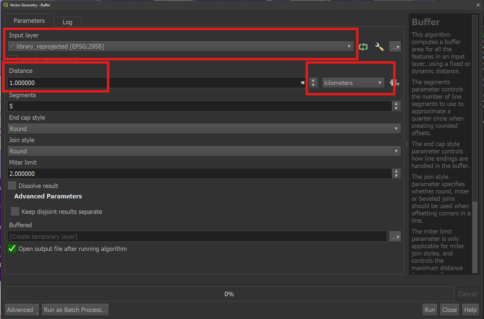
Processing toolbox → Vector Geometry → Buffer

• Specify the reprojected libraries layer as the Input layer and 1 kilometre as the Distance.

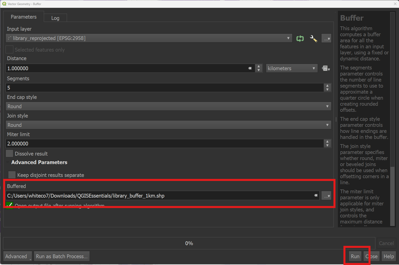
Parameters: Input layer = libraries, Distance = 1km

• Save the output layer to the data folder as library_buffer_1km.shp. Click Run.

Saving output layer

• Result: A new polygon layer representing a 1-kilometre radius around each library location.

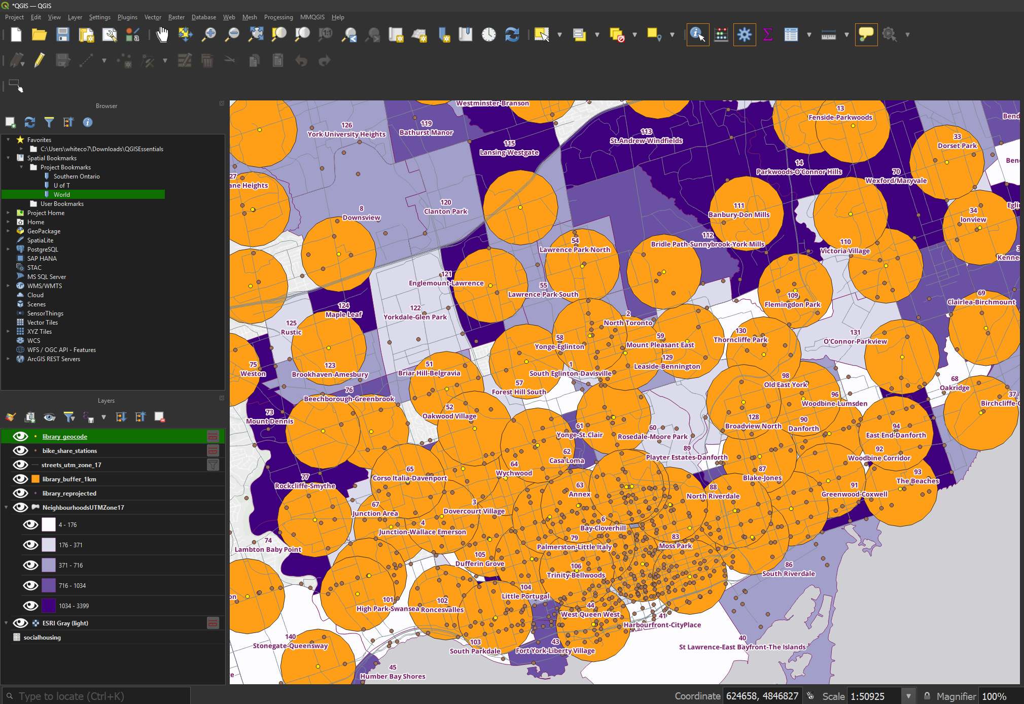
Output buffered layer in the map canvas

Summarizing data

We’ll use a geoprocessing tool to summarize how many bike share stations are within a kilometre of each library.

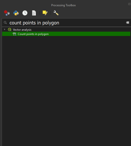
• In the Processing Toolbox, search for count points in polygon. Double-click Vector analysis → Count points in polygon to open the tool.

Vector analysis → Count points in polygon

• Specify library_buffer_1km as the Polygons parameter and bike_share_stations as the Points. Save the output as a shapefile in the data folder. Click Run.

Save output, click Run

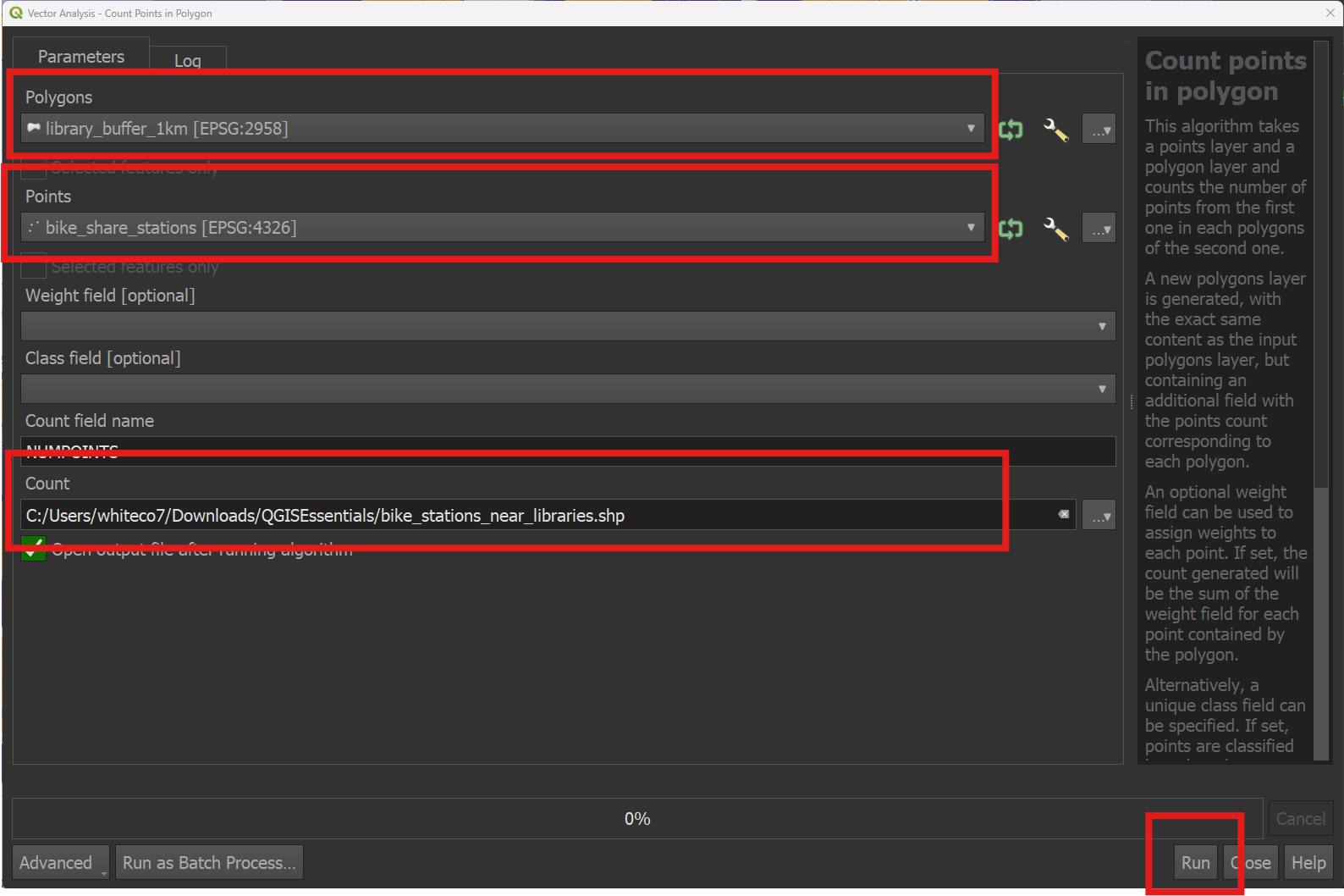
• This will output a layer with the same geometry as the buffered layer, but its attribute table will contain a new field summarizing the number of libraries found within each 1-kilometre radius of each library.

Output layer attribute table