Creating a Simple Bar Graph

3. Creating a Simple Bar Graph

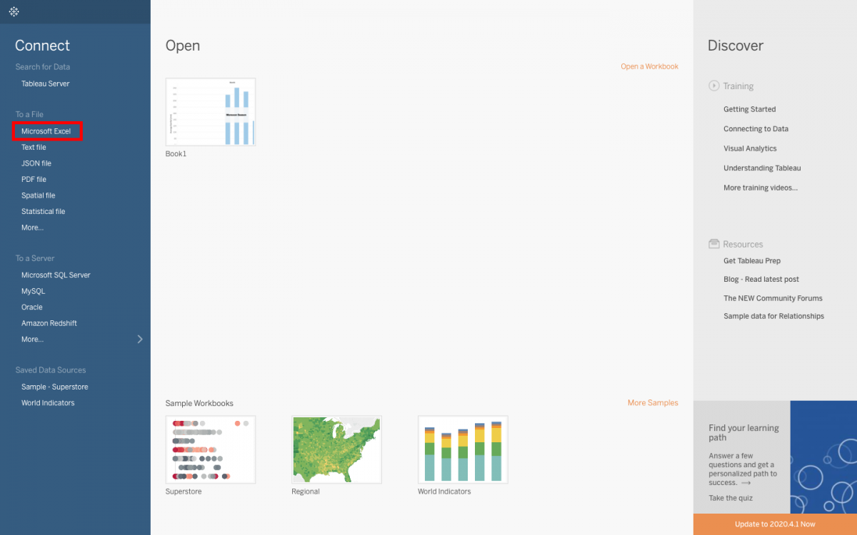
Our first dataset is an Excel file, so in Tableau, click on Excel under Connect To a File, and select the 2015RainfallByMonthByCountry.xls file. Click Open.
Connect to file menu with Microsoft Excel highlighted.

Click on Sheet 1 (at the bottom, the tab to the right of “Data Source”) to open up a worksheet and start creating your visualization.

On the left, you can see our variables listed. Tableau categorized the variables as either Dimensions or Measures, listing all the Dimensions first above the gray line, and then all the Measures below the grayline. 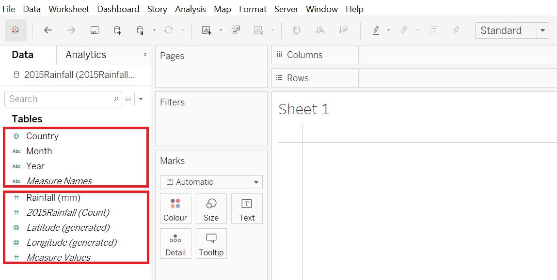Highlight of the Dimensions section at the top and the Measures section directly below it in the Sidebar

The centre area is where you will be dragging and dropping your variables onto different areas, such as rows and columns, or to vary marks like colour or size by your variable, or to filter by a variable. In terms of Tableau terminology, those areas that say filters or pages are called shelves, the marks area is called a card, and when the variables show up in those areas, they are called pills (as they are shaped like a pill). 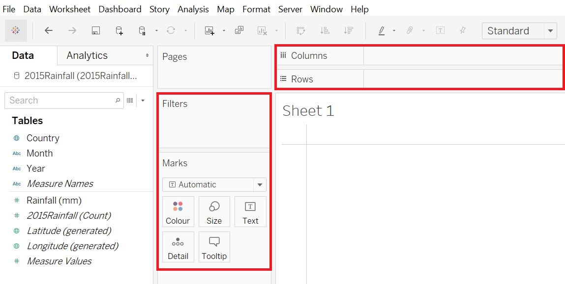The Filters and Marks section is highlighted, located to the left of the sheet. The Columns and Rows sections are also highlighted, located at the top of the sheet.

We loaded in some data that contains average monthly rainfall by country (looking at data from 1901 to 2015). So let’s create a bar graph with the month along the x-axis and average rainfall along the y-axis. Drag the Month variable (in the Dimensions section on the left) to the Columns section and Rainfall (mm) (in the Measures section on the left) variable to the Rows section. 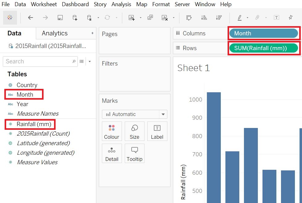Highlight of Month and rainfall variables in their original dimensions and measures location as well as in pill form in the Columns and Rows sections respectively You can see that when we dragged rainfall, it automatically summarized it by adding up all the rainfall averages for all the countries. We can change this to average. Right-click on the SUM(Rainfall (mm)) pill in the Rows section, go to the Measure (Sum) menu and pick Average. You will notice that the y-axis in the resulting graph will have changed. 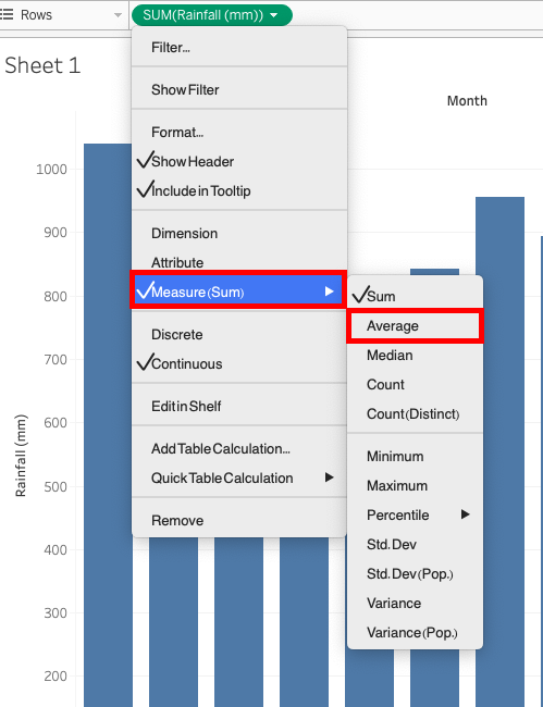SUM(Rainfall (mm)) drop down menu with Measure and Average highlighted,

Right now our graph is showing data combined for all of our countries, but let’s say we just want it to show one of them. Drag the Country variable over to the Filters shelf and select one country from the list – let’s pick India. Click OK.
Filter [Country] menu with India highlighted.

Now we have a bar graph showing the average rainfall in millimetres for India by month. 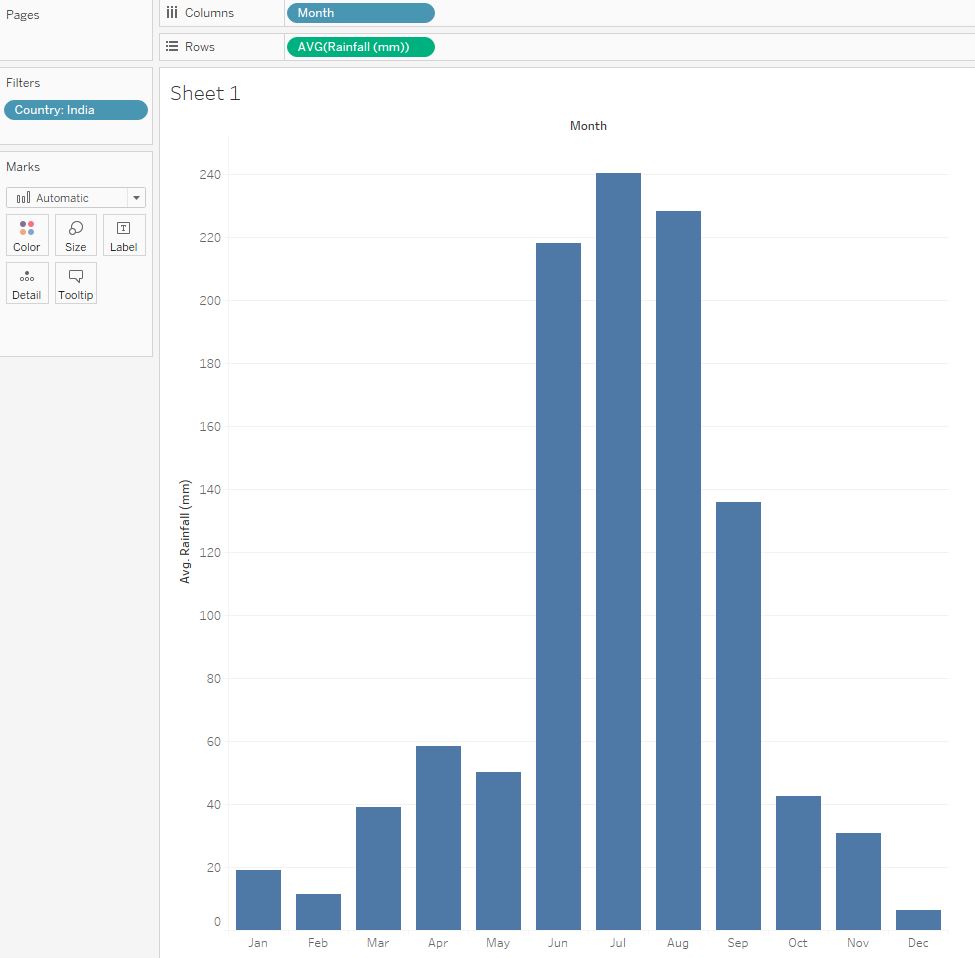Bar graph is displayed with these initial parameters. Next, let’s look at the Marks card. You should see 5 boxes labeled Color, Size, Label, Detail, and Tooltip. You can use these to customize your visualization.

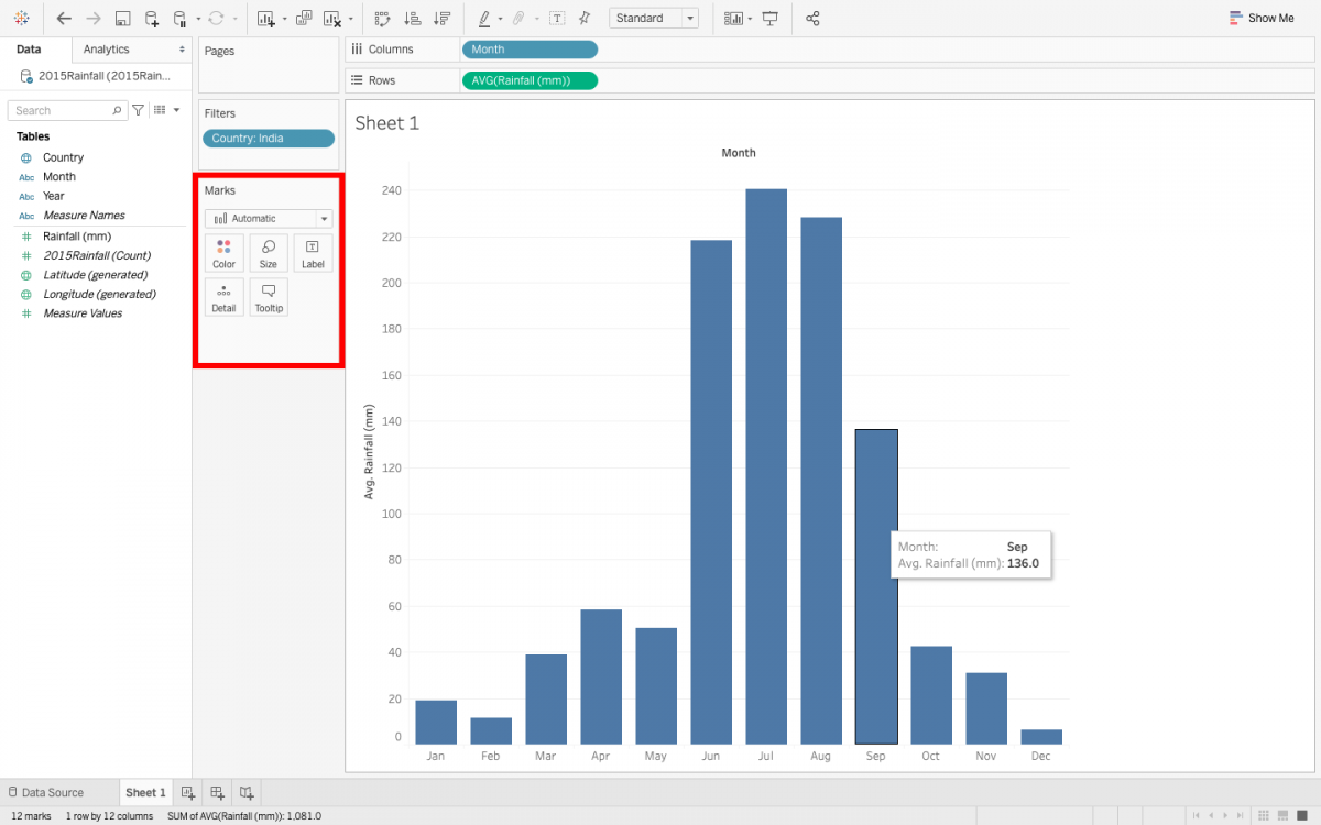
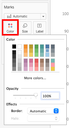
Click on Color, and change the colour of the bars to a different shade of blue.
Marks tab with Color highlighted.

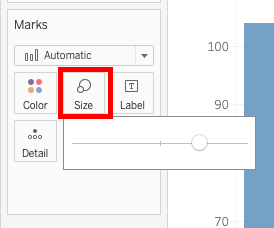
Click on Size, and use the slider to make the bars wider or narrower.
Marks tab with Size highlighted.

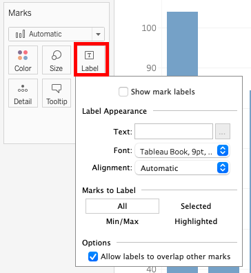
Click on Label, and select Show Mark Labels box to see the values for each bar.
Marks tab with Label highlighted.

Click on Tooltip to adjust the text that shows up in the pop-up you get when you hover over the data in your graph. Add to the bottom of the text “Data from WorldBank”. Then click on OK. Now hover over the data to see your changes. 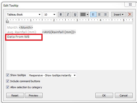Image displaying the Edit Tooltip pop-up window. 'Data From WB' is written in its textbox, underneath the default text.

You can also customize your axes. Right-click on your y-axis title, and select Edit Title… 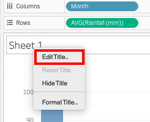Right click on y-axis option- with Edit Title highlighted.

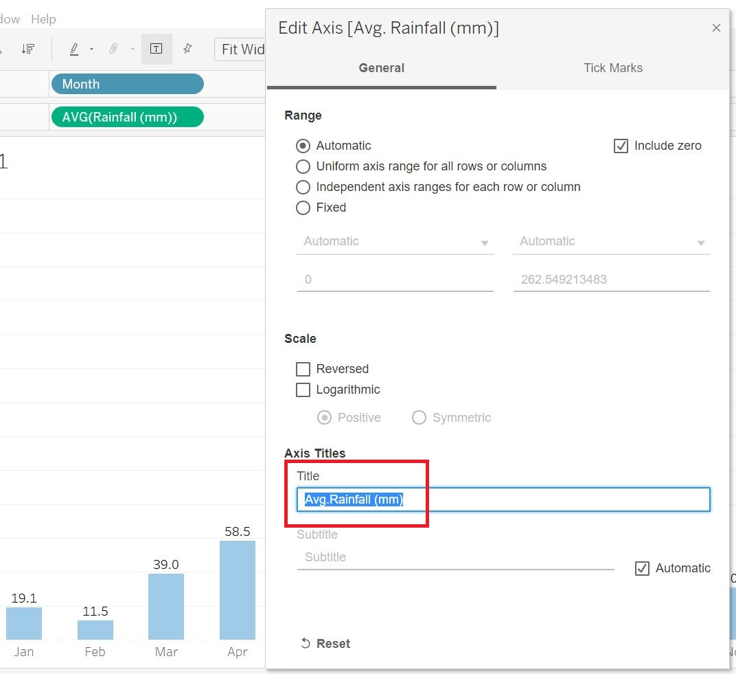
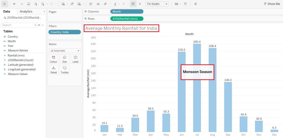
Change the title (under Axis Titles in the General tab) to write out the word “Average” instead of “Avg.” Then close the window. The change will be applied automatically, so there is no need to click a “save” button (you will notice there is no “save” button). Click the “x” in the top right-hand corner to exit the Edit Axis window. Image of the edit axis options pop-up window and the lack of an "ok" box to click

You can also annotate your visualization. Perhaps you want to point out that the summer months are Monsoon season for India, which may be why there is such a spike in average rainfall. Right-click on white space above the graph above those months and select Annotate and pick Area… Then type in “Monsoon Season”, change its font size to 12, bold it, and click OK. Now you can resize and move the box and place it where you want in the graph.

Finally, we can give our visualization a title by double-clicking on Sheet 1 at the top and replacing the text with our title “Average Monthly Rainfall for India” and click OK. Done! You have created your first visualization on Tableau Desktop.
Final bar graph is shown with the new text box and new title highlighted.
If you like this visualization and would like to learn how to save, export, or print it at this point in time, you can skip ahead to Section 9: Publishing Tableau Visualizations and Further Resources. However, you can always come back and save all of your visualizations at the end if you would prefer to proceed to the next section.

Technique: Data Visualization | Tools: Excel, Tableau